68,244 views | 00:27:17


![]()


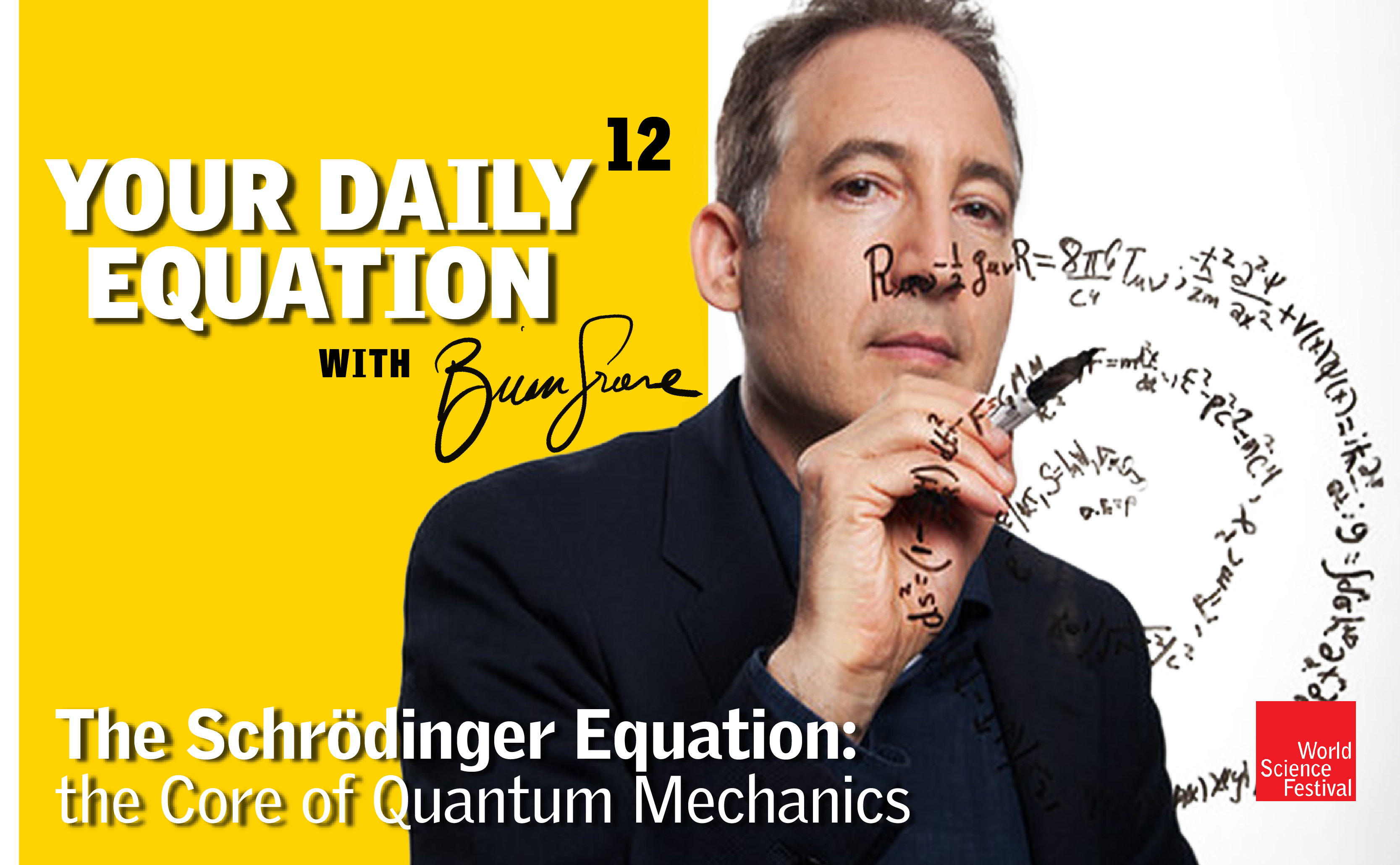


#YourDailyEquation with Brian Greene offers brief and breezy discussions of the most pivotal equations of the ages. Even if your math is a bit rusty, these accessible and exciting stories of nature and numbers will allow you to see the universe in a new way.
The series includes live Q+As that explore many of the big questions that have occupied some of the greatest thinkers of our age and yielded some of the deepest insights into the nature of reality.
Episode 16 #YourDailyEquation: Much as matter, however complicated, can be decomposed into combinations of atoms, mathematical functions, however complicated, can be decomposed into combinations of simpler functions–sines and cosines. In this episode of Your Daily Equation, Brian discusses this remarkable discovery of Joseph Fourier, which has profound applications in both math and physics.
Speaker 1:
Hi everyone, welcome to this next episode of Your Daily Equation. Yes, of course it’s that time again. Today, I’m going to focus upon a mathematical result that not only has profound implications in pure mathematics, but also has profound applications in physics as well. And in some sense, the mathematical result that we’re going to talk about is the analog, if you will, of the well known and important physical fact that any complex matter that we see in the world around us from whatever, computers to iPads, to trees, to birds, whatever, any complex matter we know can be broken down into simpler constituents, molecules or let’s just say atoms, the atoms that fill out the periodic table.
Now, what that really tells us is you can start with simple ingredients and by combining them in the right way, yield complex looking material objects. The same is basically true in mathematics when you think about mathematical function. So, it turns out as proven by Joseph Fourier mathematician born in the late 1700s that basically any mathematical function, it has to be sufficiently well behaved, and let’s put all those details to the side. Roughly, any mathematical function can be expressed as a combination, as a sum of simpler mathematical functions, and the simpler functions that people typically use and what I will focus upon here today as well, we choose sines and cosines, right, those very simple wavy shape sines and cosines.
If you adjust the amplitude of the sines and cosines and the wavelength and you combine them, that is sum them together in the right way, you can reproduce effectively any function that you start with, however complicated it may be, it can be expressed in terms of these simple ingredients, the simple function sines and cosines. That’s the basic idea. Let’s just take a quick look at how you actually do that in practice.
So, the subject here is Fourier series and I think the simplest way to get going is to give an example straight off the bat, and for that I’m going to use a little bit of graph paper so I can try to keep this as neat as possible. So, let’s imagine that I have a function and because I’m going to be using sines and cosines, which we all know they repeat, these are periodic functions. I’m going to choose a particular periodic function to begin with to have a fighting chance of being able to express in terms of sines and cosines, and I’ll choose a very simple periodic function. I’m not trying to be particularly creative here. Many people who are teaching this subject start off with this example. It’s the square wave, and you’ll note that I could just keep on doing this.
This is the repetitive periodic nature of this function, but I’ll stop here. And the goal right now is to see how this particular shape, this particular function can be expressed in terms of sines and cosines. Indeed, it will just be in terms of sines because of the way that I have drawn this here. Now, if I was to come to you and say challenge you to take a single sine wave and approximate this red square wave, what would you do? Well, I think you’d probably do something like this. You’d say, let me look at a sine wave, whoops, definitely that’s not a sine wave. The sine wave that comes up, swings around down here, swings back over here and so forth and carries out. I won’t bother writing the periodic versions to the right or to the left. I’ll just focus upon them, that one interval right there.
Now, that blue sine wave, it’s not a bad approximation to the red square wave, you’d never would confuse one for the other, but you seem to be heading in the right direction. But then if I challenge you to go a little bit further and add in another sine wave to try to make the combined wave a little bit closer to the square red shape, what would you do? Well, here are the things that you can adjust. You can adjust how many wiggles the sine wave has that as its wavelength and you can adjust the amplitude of the new piece that you add in. So, let’s do that.
So imagine you add in, say a little piece that looks like this. Maybe it comes up like this, like that. Now, if you add it together, the red, not the red. If you add it together the green and the blue, certainly you wouldn’t get hot pink, but let me use hot pink for their combination. Well in this part, the green is going to push the blue up a little bit when you add them together. In this region, the green is going to pull the blue down, so it’s going to push this part of the wave a little closer to the red, and in this region it’s going to pull the blue downward a little closer to red as well. So, that seems like a good additional wave to add in. Let me clean this, add the guy up and actually do that addition.
So, if I do that, it’ll push it up in this region, pull it down in this region, up in this region, similarly down in here and something like that. So now the pink is a little bit closer to the red and you could at least imagine that if I was to judiciously choose the height of additional sine waves and the wavelength, how quickly they are oscillating up and down that by appropriately choosing those ingredients, I could get closer and closer to the red square wave. And indeed I can show you, I can’t do it by hand obviously, but I can show you up here on the screen an example obviously done with a computer, and you see that if we add the first and second sine waves together, you get something that’s pretty close as we have in my hand drawn to the square wave.
But in this particular case it goes up to adding 50 distinct sine waves together with various amplitudes and various wave lengths. And you see that that particular color, it’s the dark orange gets really close to being a square wave. So that’s the basic idea, add together enough sines and cosines and you can reproduce any wave shape that you like. Okay, so that’s the basic idea in pictorial form. But now, let me just write down some of the key equations and therefore let me start with a function.
Any function called F of X, and I’m going to imagine that it’s periodic in the interval from minus L to L. So, not minus L to minus L, let me get rid of that guy there from minus L to L. What that means is its value at minus L and its value at L will be the same, and then it just periodically continues the same wave shape just shifted over by the amount to L along the X axis. So again, just so I can give you a picture for that before I write down the equation. So, imagine then that I have my axis here and let’s for instance call this point minus L and this guy on the symmetric side, I’ll call plus L, and let me just choose some wave shape in there. I’ll again use red.
So imagine, I don’t know, it comes up and I’m just drawing some random shape. And the idea is that it’s periodic, so I’m not going to try to copy that by hand. Rather, I’ll use the ability, I believe to copy and then paste this over. Oh look at that, that worked out quite well. So as you can see, it has over the interval, a full interval of size 2L. It just repeats and repeats and repeats. That’s my function, my general guy F of X. And the claim is that this guy can be written in terms of sines and cosines, and only be a little bit careful about the arguments of the sines and cosines. And the claim is, well maybe I’ll write down the theorem and then I’ll explain each of the terms that might be the most efficient way to do it.
The theorem that Joseph Fourier proves for us is that F of X can be written … Well, why am I changing color? I think that’s a little bit stupidly confusing. So, let me use red for F of X. And now let me use blue say when I write in terms of sines and cosines. So, it can be written as a number, just a coefficient, usually written [inaudible 00:09:39] divided by two plus, now here are the sums of the sines and co-sine, so N equals one to infinity, AN, I’ll start with a co-sine part, co-sine. And here look at the argument N PI X over L. I’ll explain why in half a second it takes that particular strange look and form, plus a summation N equals one to infinity, BN times sine of N PI X over L. Boy, that is squeezed in there, so I’m actually going to use my ability to just squeeze this down a little bit, move it over and it looks a little bit better.
Okay. Now, why do I have this curious looking argument? I’ll look at the co-sine one. Y co-sine of N PI X over L. Well look if F of X has the property, that F of X equals F of X plus 2L, right? That’s what it means that it repeats every 2L units left or right, then that has to be the case at the cosines and sines that use also repeat if X goes to X plus 2L, and let’s take a look at that. So, if I have co-sine of N PI X over L, what happens if I replace X by X plus 2L? Well let me stick that right inside. So, I’ll get co-sine of N PI X plus 2L divided by L. What does that equal? Well, I get co-sine of N PI X over L plus I get N PI times 2L over L, the L’s cancel and I get 2NPI.
And notice, we all know that co-sine of N PI X over L, a co-sine of theta plus 2PI times an integer, doesn’t change the value of the co-sine and doesn’t change and hide the sine. So, it’s this equality, which is why I use this N PI X over L as it ensures that my cosines and sines have the same periodicity as the function F of X itself. So, that’s why I take this particular form. But let me erase all this stuff here because I just want to go back to the theorem now that you understand why it looks that way. I hope you don’t mind. When I do this in class on a blackboard, it’s at this point that the students say, “Wait, I haven’t written it all down yet,” but you can rewind if you wanted to, so you could go back. So, I’m not going to worry about that.
But I want to finish off the equation, the theorem, because what Fourier does gives us an explicit formula for A0, AN and BN. And that is an explicit formula in the case of the ANs and BNs for how much of this particular co-sine and how much of this particular sine, sine N PI X of other co-sine of N PI X over L. And here is the result. So let me write it in a more vibrant color. So A0, it’s one over L the integral from minus L to L of F of X, DX. AN is one over L integral from minus L to L, F of X times co-sine of N PI X over L, DX. And BN is one of over L integral minus L to L, F of X times sine of N PI X over L.
Now again, for those of you who are rusty on your calculus or never took it, sorry that this may at this stage be a little bit opaque. But the point is that an integral is nothing but a fancy kind of summation. So, what we have here is an algorithm that Fourier gives us for determining the weight of the various sines and cosines that are on the right hand side and these integrals are something that given the function F you can sort of, just not sort of, you can plug it in to this formula and get the values of A0, AN, and BN that you need to plug into this expression in order to have the equality between the original function and this combination of sines and cosines.
Now, for those of you who are interested to understand how you prove this, it’s actually so straightforward to proof. You simply integrate F of X against a cosine or a sine, and those of you who remember your calculus will recognize that when you integrate a cosine against a cosine that will be zero if their arguments are different, and that’s why the only contribution we’ll get is for the value of AN when this is equal to N. And similarly for the sines, the only non-zero if you integrate F of X against a sine will be when the argument of that agrees with the sine here. And that’s why this N picks out this N over here.
So anyway, that’s the rough idea of the proof, if you know your calculus, remember that cosines and sines yield an orthogonal set of functions. You can prove this, but my goal here is not to prove it. My goal here is to show you this equation and for you to have an intuition that it is formalizing what we did in our little toy example earlier where we by hand had to pick the amplitudes and the wavelengths of the various sines, waves that we were putting together. Now, this formula tells you exactly how much of a given say, sine wave to put in given the function F of X, you can calculate it with this beautiful little formula.
So, that’s the basic idea of Fourier series. Again, it’s incredibly powerful because sines and cosines are so much easier to deal with than this arbitrary say wave shape that I wrote down as our motivating shape to begin with. It’s so much easier to deal with waves that have a well understood property both from the standpoint of functions and in terms of their graphs as well. The other utility of the Fourier series for those of you who are interested is that it allows you to solve certain differential equations much more simply than you would otherwise be able to do if they’re linear differential equations and you can solve them in terms of sines and cosines. You can then combine the sines and cosines to get any initial wave shape that you like, and therefore you might’ve thought you were limited to the nice periodic sines and cosines that had this nice simple, wavy shape, but you can get something that looks like this out of sines and cosines, so you can really get anything out of it at all.
The other thing that I don’t have time to discuss, but those of you who perhaps have taken some calculus will note that you can go a little bit further than Fourier series to something called a Fourier transform where you turn the coefficients AN and BN themselves into a function. The function is a weighting function which tells you how much of a given amount of sine and cosine, you need to put together in the continuous case when you let L go to infinities. These are details that if you haven’t studied, the subject may go by too quickly, but I’m mentioning it because it turns out that Heisenberg’s uncertainty principle and quantum mechanics emerges from these very kinds of considerations.
And of course Joseph Fourier was not thinking about quantum mechanics or the uncertainty principle, it’s a remarkable fact that I’ll mention again when I talk about the uncertainty principle which I’ve not done in this Your Daily Equation series, but I will at some point in the not too distant future, but it turns out that the uncertainty principle is nothing but a special case of Fourier series, an idea that mathematically was spoken of 150 years or so earlier than the uncertainty principle itself is just beautiful confluence of mathematics that’s derived and thought about in one context and yet when properly understood, gives you deep insights into the fundamental nature of matter as described by quantum physics.
Okay. So, that’s all I wanted to do today, the fundamental equation given to us by Joseph Fourier in the form of the Fourier series. So, until next time, that is Your Daily Equation.
#YourDailyEquation with Brian Greene offers brief and breezy discussions of the most pivotal equations of the ages. Even if your math is a bit rusty, these accessible and exciting stories of nature and numbers will allow you to see the universe in a new way.
The series includes live Q+As that explore many of the big questions that have occupied some of the greatest thinkers of our age and yielded some of the deepest insights into the nature of reality.
Episode 16 #YourDailyEquation: Much as matter, however complicated, can be decomposed into combinations of atoms, mathematical functions, however complicated, can be decomposed into combinations of simpler functions–sines and cosines. In this episode of Your Daily Equation, Brian discusses this remarkable discovery of Joseph Fourier, which has profound applications in both math and physics.

Brian Greene is a professor of physics and mathematics at Columbia University, and is recognized for a number of groundbreaking discoveries in his field of superstring theory. His books, The Elegant Universe, The Fabric of the Cosmos, and The Hidden Reality, have collectively spent 65 weeks on The New York Times bestseller list.
Read MoreSpeaker 1:
Hi everyone, welcome to this next episode of Your Daily Equation. Yes, of course it’s that time again. Today, I’m going to focus upon a mathematical result that not only has profound implications in pure mathematics, but also has profound applications in physics as well. And in some sense, the mathematical result that we’re going to talk about is the analog, if you will, of the well known and important physical fact that any complex matter that we see in the world around us from whatever, computers to iPads, to trees, to birds, whatever, any complex matter we know can be broken down into simpler constituents, molecules or let’s just say atoms, the atoms that fill out the periodic table.
Now, what that really tells us is you can start with simple ingredients and by combining them in the right way, yield complex looking material objects. The same is basically true in mathematics when you think about mathematical function. So, it turns out as proven by Joseph Fourier mathematician born in the late 1700s that basically any mathematical function, it has to be sufficiently well behaved, and let’s put all those details to the side. Roughly, any mathematical function can be expressed as a combination, as a sum of simpler mathematical functions, and the simpler functions that people typically use and what I will focus upon here today as well, we choose sines and cosines, right, those very simple wavy shape sines and cosines.
If you adjust the amplitude of the sines and cosines and the wavelength and you combine them, that is sum them together in the right way, you can reproduce effectively any function that you start with, however complicated it may be, it can be expressed in terms of these simple ingredients, the simple function sines and cosines. That’s the basic idea. Let’s just take a quick look at how you actually do that in practice.
So, the subject here is Fourier series and I think the simplest way to get going is to give an example straight off the bat, and for that I’m going to use a little bit of graph paper so I can try to keep this as neat as possible. So, let’s imagine that I have a function and because I’m going to be using sines and cosines, which we all know they repeat, these are periodic functions. I’m going to choose a particular periodic function to begin with to have a fighting chance of being able to express in terms of sines and cosines, and I’ll choose a very simple periodic function. I’m not trying to be particularly creative here. Many people who are teaching this subject start off with this example. It’s the square wave, and you’ll note that I could just keep on doing this.
This is the repetitive periodic nature of this function, but I’ll stop here. And the goal right now is to see how this particular shape, this particular function can be expressed in terms of sines and cosines. Indeed, it will just be in terms of sines because of the way that I have drawn this here. Now, if I was to come to you and say challenge you to take a single sine wave and approximate this red square wave, what would you do? Well, I think you’d probably do something like this. You’d say, let me look at a sine wave, whoops, definitely that’s not a sine wave. The sine wave that comes up, swings around down here, swings back over here and so forth and carries out. I won’t bother writing the periodic versions to the right or to the left. I’ll just focus upon them, that one interval right there.
Now, that blue sine wave, it’s not a bad approximation to the red square wave, you’d never would confuse one for the other, but you seem to be heading in the right direction. But then if I challenge you to go a little bit further and add in another sine wave to try to make the combined wave a little bit closer to the square red shape, what would you do? Well, here are the things that you can adjust. You can adjust how many wiggles the sine wave has that as its wavelength and you can adjust the amplitude of the new piece that you add in. So, let’s do that.
So imagine you add in, say a little piece that looks like this. Maybe it comes up like this, like that. Now, if you add it together, the red, not the red. If you add it together the green and the blue, certainly you wouldn’t get hot pink, but let me use hot pink for their combination. Well in this part, the green is going to push the blue up a little bit when you add them together. In this region, the green is going to pull the blue down, so it’s going to push this part of the wave a little closer to the red, and in this region it’s going to pull the blue downward a little closer to red as well. So, that seems like a good additional wave to add in. Let me clean this, add the guy up and actually do that addition.
So, if I do that, it’ll push it up in this region, pull it down in this region, up in this region, similarly down in here and something like that. So now the pink is a little bit closer to the red and you could at least imagine that if I was to judiciously choose the height of additional sine waves and the wavelength, how quickly they are oscillating up and down that by appropriately choosing those ingredients, I could get closer and closer to the red square wave. And indeed I can show you, I can’t do it by hand obviously, but I can show you up here on the screen an example obviously done with a computer, and you see that if we add the first and second sine waves together, you get something that’s pretty close as we have in my hand drawn to the square wave.
But in this particular case it goes up to adding 50 distinct sine waves together with various amplitudes and various wave lengths. And you see that that particular color, it’s the dark orange gets really close to being a square wave. So that’s the basic idea, add together enough sines and cosines and you can reproduce any wave shape that you like. Okay, so that’s the basic idea in pictorial form. But now, let me just write down some of the key equations and therefore let me start with a function.
Any function called F of X, and I’m going to imagine that it’s periodic in the interval from minus L to L. So, not minus L to minus L, let me get rid of that guy there from minus L to L. What that means is its value at minus L and its value at L will be the same, and then it just periodically continues the same wave shape just shifted over by the amount to L along the X axis. So again, just so I can give you a picture for that before I write down the equation. So, imagine then that I have my axis here and let’s for instance call this point minus L and this guy on the symmetric side, I’ll call plus L, and let me just choose some wave shape in there. I’ll again use red.
So imagine, I don’t know, it comes up and I’m just drawing some random shape. And the idea is that it’s periodic, so I’m not going to try to copy that by hand. Rather, I’ll use the ability, I believe to copy and then paste this over. Oh look at that, that worked out quite well. So as you can see, it has over the interval, a full interval of size 2L. It just repeats and repeats and repeats. That’s my function, my general guy F of X. And the claim is that this guy can be written in terms of sines and cosines, and only be a little bit careful about the arguments of the sines and cosines. And the claim is, well maybe I’ll write down the theorem and then I’ll explain each of the terms that might be the most efficient way to do it.
The theorem that Joseph Fourier proves for us is that F of X can be written … Well, why am I changing color? I think that’s a little bit stupidly confusing. So, let me use red for F of X. And now let me use blue say when I write in terms of sines and cosines. So, it can be written as a number, just a coefficient, usually written [inaudible 00:09:39] divided by two plus, now here are the sums of the sines and co-sine, so N equals one to infinity, AN, I’ll start with a co-sine part, co-sine. And here look at the argument N PI X over L. I’ll explain why in half a second it takes that particular strange look and form, plus a summation N equals one to infinity, BN times sine of N PI X over L. Boy, that is squeezed in there, so I’m actually going to use my ability to just squeeze this down a little bit, move it over and it looks a little bit better.
Okay. Now, why do I have this curious looking argument? I’ll look at the co-sine one. Y co-sine of N PI X over L. Well look if F of X has the property, that F of X equals F of X plus 2L, right? That’s what it means that it repeats every 2L units left or right, then that has to be the case at the cosines and sines that use also repeat if X goes to X plus 2L, and let’s take a look at that. So, if I have co-sine of N PI X over L, what happens if I replace X by X plus 2L? Well let me stick that right inside. So, I’ll get co-sine of N PI X plus 2L divided by L. What does that equal? Well, I get co-sine of N PI X over L plus I get N PI times 2L over L, the L’s cancel and I get 2NPI.
And notice, we all know that co-sine of N PI X over L, a co-sine of theta plus 2PI times an integer, doesn’t change the value of the co-sine and doesn’t change and hide the sine. So, it’s this equality, which is why I use this N PI X over L as it ensures that my cosines and sines have the same periodicity as the function F of X itself. So, that’s why I take this particular form. But let me erase all this stuff here because I just want to go back to the theorem now that you understand why it looks that way. I hope you don’t mind. When I do this in class on a blackboard, it’s at this point that the students say, “Wait, I haven’t written it all down yet,” but you can rewind if you wanted to, so you could go back. So, I’m not going to worry about that.
But I want to finish off the equation, the theorem, because what Fourier does gives us an explicit formula for A0, AN and BN. And that is an explicit formula in the case of the ANs and BNs for how much of this particular co-sine and how much of this particular sine, sine N PI X of other co-sine of N PI X over L. And here is the result. So let me write it in a more vibrant color. So A0, it’s one over L the integral from minus L to L of F of X, DX. AN is one over L integral from minus L to L, F of X times co-sine of N PI X over L, DX. And BN is one of over L integral minus L to L, F of X times sine of N PI X over L.
Now again, for those of you who are rusty on your calculus or never took it, sorry that this may at this stage be a little bit opaque. But the point is that an integral is nothing but a fancy kind of summation. So, what we have here is an algorithm that Fourier gives us for determining the weight of the various sines and cosines that are on the right hand side and these integrals are something that given the function F you can sort of, just not sort of, you can plug it in to this formula and get the values of A0, AN, and BN that you need to plug into this expression in order to have the equality between the original function and this combination of sines and cosines.
Now, for those of you who are interested to understand how you prove this, it’s actually so straightforward to proof. You simply integrate F of X against a cosine or a sine, and those of you who remember your calculus will recognize that when you integrate a cosine against a cosine that will be zero if their arguments are different, and that’s why the only contribution we’ll get is for the value of AN when this is equal to N. And similarly for the sines, the only non-zero if you integrate F of X against a sine will be when the argument of that agrees with the sine here. And that’s why this N picks out this N over here.
So anyway, that’s the rough idea of the proof, if you know your calculus, remember that cosines and sines yield an orthogonal set of functions. You can prove this, but my goal here is not to prove it. My goal here is to show you this equation and for you to have an intuition that it is formalizing what we did in our little toy example earlier where we by hand had to pick the amplitudes and the wavelengths of the various sines, waves that we were putting together. Now, this formula tells you exactly how much of a given say, sine wave to put in given the function F of X, you can calculate it with this beautiful little formula.
So, that’s the basic idea of Fourier series. Again, it’s incredibly powerful because sines and cosines are so much easier to deal with than this arbitrary say wave shape that I wrote down as our motivating shape to begin with. It’s so much easier to deal with waves that have a well understood property both from the standpoint of functions and in terms of their graphs as well. The other utility of the Fourier series for those of you who are interested is that it allows you to solve certain differential equations much more simply than you would otherwise be able to do if they’re linear differential equations and you can solve them in terms of sines and cosines. You can then combine the sines and cosines to get any initial wave shape that you like, and therefore you might’ve thought you were limited to the nice periodic sines and cosines that had this nice simple, wavy shape, but you can get something that looks like this out of sines and cosines, so you can really get anything out of it at all.
The other thing that I don’t have time to discuss, but those of you who perhaps have taken some calculus will note that you can go a little bit further than Fourier series to something called a Fourier transform where you turn the coefficients AN and BN themselves into a function. The function is a weighting function which tells you how much of a given amount of sine and cosine, you need to put together in the continuous case when you let L go to infinities. These are details that if you haven’t studied, the subject may go by too quickly, but I’m mentioning it because it turns out that Heisenberg’s uncertainty principle and quantum mechanics emerges from these very kinds of considerations.
And of course Joseph Fourier was not thinking about quantum mechanics or the uncertainty principle, it’s a remarkable fact that I’ll mention again when I talk about the uncertainty principle which I’ve not done in this Your Daily Equation series, but I will at some point in the not too distant future, but it turns out that the uncertainty principle is nothing but a special case of Fourier series, an idea that mathematically was spoken of 150 years or so earlier than the uncertainty principle itself is just beautiful confluence of mathematics that’s derived and thought about in one context and yet when properly understood, gives you deep insights into the fundamental nature of matter as described by quantum physics.
Okay. So, that’s all I wanted to do today, the fundamental equation given to us by Joseph Fourier in the form of the Fourier series. So, until next time, that is Your Daily Equation.