165,065 views | 00:34:40

![]()


Join us for #YourDailyEquation with Brian Greene. Every Mon – Fri at 3pm EDT, Brian Greene will offer brief and breezy discussions of pivotal equations. Even if your math is a bit rusty, tune in for accessible and exciting stories of nature and numbers that will allow you to see the universe in a new way.
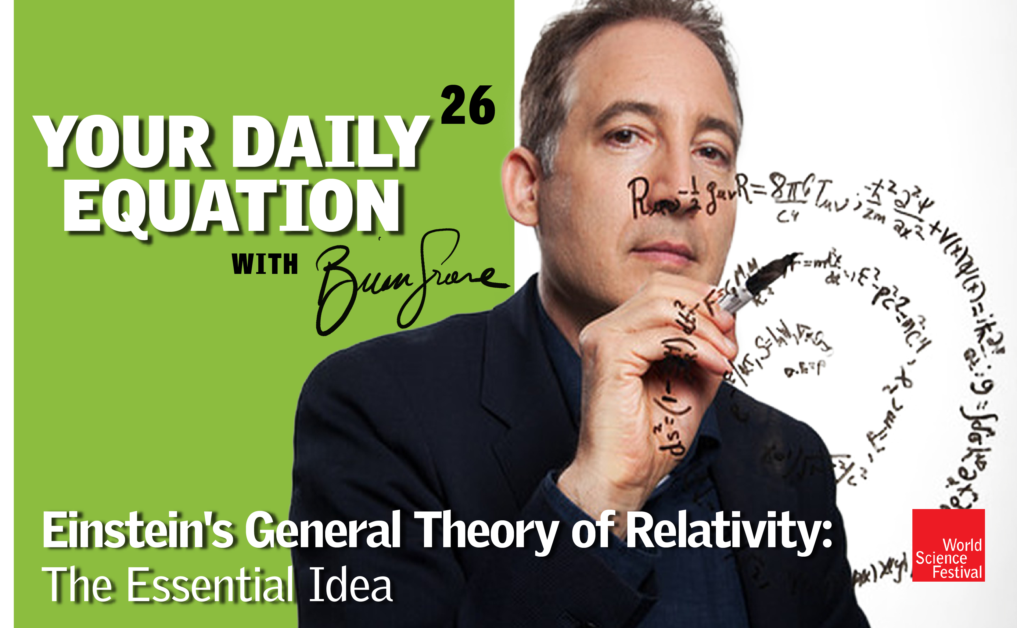
Episode 27 #YourDailyEquation: In his general theory of relativity, Einstein described gravity in terms of the curvature of space and time. Join Brian Greene for an introduction to the mathematics of curvature, which Einstein used to fashion his gravitational field equations.
Speaker 1:
Hey everyone. Welcome to this next episode of Your Daily Equation. And today the focus will be on the concept of curvature. Curvature, why curvature? Well, as we saw in an earlier episode of Your Daily Equation and perhaps on your own, even if you didn’t see any previous episodes, when Einstein formulated his new description of gravity, the general theory of relativity, he made profound use of the notion that space and time can be curved and through that curvature objects are coaxed, nudged to travel along particular trajectories that in the older language we would describe as the gravitational pole, the force of attraction of another body on the object that we are investigating. And Einstein’s description, it’s actually the curvature of space that is guiding the object and its motion.
So again, just to put us on the same page, a visual that I’ve used before, but I think it’s certainly a good one, here we have space, three dimensions, hard to picture. So I’m going to go to a two dimensional version that captures all of the ideas. See that space is nice and flat when there’s nothing there. But when I bring in the Sun, the fabric of space curves, and similarly, if you look in the vicinity of the Earth, the Earth too curves its environment and the Moon, as you see is kept in orbit, because it’s rolling along a valley in the curved environment that the Earth creates. So the Moon is being pushed around into orbit by grooves in the curved environment that the Earth, in this particular case, creates. And the Earth is kept an orbit for the same reason, it stays in orbit around the Sun because the Sun curves the environment and the Earth is nudged into orbit by that particular shape.
So with that new way of thinking about gravity, where space and time are intimate participants in the physical phenomena, they’re not just an inert backdrops, not just that things are moving through a container. We see an Einstein’s vision that the curvature of space and time. Time curvature is a tricky concept, we’ll come to it at some point, but just think in terms of space, it’s easier. So the curvature of the environment is what exerts this influence that causes objects to move in the trajectories that they do. But of course, to make this precise, not just animation and pictures, if you want to make this precise, you need the mathematical means for talking about curvature with precision. And in Einstein’s day, he was able to thankfully draw upon earlier work that had been done by people like Gauss and Lobachevsky and Riemann in particular, Einstein was able to grab these mathematical developments from the 1800s, reshaped them in a manner that allowed them to be relevant for the curvature of space time for how gravity is manifested through the curvature of space time.
But thankfully for Einstein, he didn’t have to develop all that mathematics from scratch. And so what we’re going to do today is talk a little bit about… I’m tethered here by a wire, unfortunately, because, 13%. You may say, why am I always so low in power? I don’t know. But I’m going to take this out for a bit and see what happens if it gets too low, I’ll plug it back in. Anyway. So we’re talking about then curvature and I think I’m going to cover this in two steps. Maybe I’ll do both steps today, but time is short. So I don’t know if I will get to it.
I’d like to talk first about just the intuitive idea. And then I would like to give you the actual mathematical formalism for those who are interested, But having the intuitive idea in mind is pretty vital, pretty important. So what’s the idea? Well, to get to the intuitive idea, I’m going to start with something that at first sight won’t seem to have much to do with curvature at all. I’m going to make use of what I would like to call and what people typically do call, a notion of parallel transport or parallel translation. What does that mean? Well, I can show you what it means with a picture. So if you have a vector say in the X, Y plane, some arbitrary vector is sitting there at the origin. If I asked you to move that vector to some other location on the plane, and I said, just be certain to keep it parallel to itself, you know exactly how to do that.
You grab hold of the vector and in Notability, there’s a very nice way of doing it. I can copy it over here. I think. Paste. Good. And now look what I can do. Well, that’s beautiful. So I can move it all around the plane. This is fun. And I can bring it right to this specified location. And there it is. I’ve parallel transported the initial vector from the initial point to the final point. Now here’s the interesting thing that is obvious on the plane, but will be less obvious in other shapes. If I were to paste this again, good, there’s the vector again, let’s say I take a completely different trajectory. I move it like this, like this, like this, and I get to the same spot. I’ll put it right next to it, if I could. Yeah. You’ll note that the vector that I get at the green dot is completely independent of the path that I took.
I just showed that to you right now. I’ve parallel transported along two different trajectories. And yet when I got to the green point, the resulting vector was identical. But that quality, the path independence of parallel translation of vectors in general does not hold. In fact on a curved surface, it generally does not hold. And let me give you an example and I’ve taken my son’s basketball, he hasn’t doesn’t know this. I hope it’s okay with him. And I should have a pen. I don’t have a pen around? That’s too bad. I was going to draw on the basketball. I could have sworn I had a pen around here. I do have a pen. Aha. It’s over here. All right. So here’s what I’m going to do. I’m going to play the same game. But in this particular case, what I’m going to do is in fact, let me do this on the plane too.
So let me bring this back up here. Let me just do one more example of this. Here’s the journey that I’m going to take. I’m going to take a vector and I’m going to parallel translate it on a loop. Here I go. I’m doing it right here on the plane, on a loop and I’m bringing it back. And just as we found with the green dot P, if we’re going to loop back to the original location, again, the new vector points in the same direction as the original. Let’s undertake that kind of a journey on the sphere. How I’m going to do that? Well, I’m going to begin with the vector over here. Can you see that? I got to go higher up. This point over here. And man, that really does not write at all. I think you have some liquid here. Maybe there’s a contact lens fluid. Let’s see if I can get it to work. Sort of. Anyway, you’ll remember. Will you remember? How am I going to do this? Well, if I had a piece of tape or something, I could use that.
Gosh, I don’t know. Anyway, so here we go. We’re all good. So anyway, can you see that at all? That’s the direction in which… I know what I’ll do. I’ll take this guy over here. I’ll use my Apple Pencil. There’s my vector. Okay. It’s at this spot right here, pointing in that direction. Okay. So you will recall that it is pointing right toward the window. Now what I’m going to do is I’m going to take this vector. I’m going to move it along a journey. The journey, here’s the journey. Let me just share the journey. I’m going to go along this black line here til I get to this equator. I’m then going to move along the equator until I get to this point over here. And then I come back up. So a nice big loop. Did I do that high enough?
Start here, down to the equator, over to this black line over here and then up here. All right. Now let’s do that. Here’s my guy initially pointing like this. So there it is. My finger and the vector are parallel. They’re at the same spot. All right, here we go. So I take this, I move it down. I am parallel transporting it down to this location over here, I then move to the other spot over here. This is harder to do. And then up, I come here. Now for this to really impact, I need to show you that initial vector. So hang on one second. I’m just going to see if I can get myself some tape. I do. Here we go. Beautiful. All right, guys. I’m coming back. Hang on. Alrighty. Perfect. All right. Sorry about that. What I’m going to do is I’m going to take a piece of tape. All right.
Yeah, that’s good. Nothing like a little bit of tape. All right. So here is my initial vector. It is pointing in that direction over here. Okay. So now let’s play this game again. All right. So I take this one over here. I start like that. And now parallel translating along this black parallel to itself. I get to the equator. Okay. I’m now going to parallel transport along the equator till I get to this location. And now I’m going to parallel transport along that black and notice it’s not… Whoops. Can you see it? It’s pointing in that direction as opposed to this direction. I’m now right angles. In fact, I’m going to do this one more time just to make this even sharper, make a thinner piece of tape. Aha. Look at that. All right. We’re cooking with gas here. All right. So here’s my initial vector.
Now it really has a direction associate with it. It’s right in there. Can you see it? That’s my initial one. Maybe I’ll take this right up close. Here we go. All right. We parallel transport, vector is parallel to itself. Parallel, parallel, parallel. Let me get down here to the equator. I keep going too low. Then I go along the equator until I get to this one over here, that black line, I’m going to go up the black line parallel to itself. And look, I’m now pointing in a different direction from the initial vector. The initial vector is this way and that new vector is that way. So I should put it at this location. So my new vectors this way and my old vector is that way.
So that was a long winded way of showing that on a sphere, a curved surface, when you parallel transport a vector, it doesn’t come back pointing in the same direction. So what that means is we have a diagnostic tool, if you will. So we have a tool, a diagnostic, a diag… Come on. A diag…. My God. Let’s see if we get through this diagnostic tool for curvature, which is this, path dependence of parallel transport.
So on a flat surface, like the plane, when you move from location to location, it doesn’t matter the path you take when you’re moving a vector as we showed on the plane, using the iPad and Notability from here and here, all the vectors are pointing the same direction, regardless of the path that you took to move the old vectors, say to the new vector. The old vector moved along this path to the new vector. You can see they’re right on top of each other, pointing in the same direction. But on the sphere we played the same game and they do not point in the same direction. So that is the intuitive way that we are going to quantify curvature. We’re going to quantify it in essence, by moving vectors along various trajectories and comparing the old and the new and the degree of difference between the parallel transported vector and the original. The degree of difference will capture the degree of curvature. The amount of curvature is the amount of the difference between those factors.
All right. Now, if you want to make this… So look, that’s really the intuitive idea right here. And now let me just, I’m going to record what the equation looks like. And yeah, I think I’m running out of time for today. For in a subsequent episode, I will take you through the mathematical manipulations that will yield this equation, but let me just set up the essence of it right here. So first off you have to bear in mind that you have to on a curve surface, define what you mean by parallel.
You see on the plane, the plane is misleading because these vectors, when you’re moving around on the surface, there isn’t any intrinsic curvature to the space. So it’s very easy to compare the direction of a vector, say at this spot with the direction of a vector of that spot. But if you do this on this sphere. Let me bring this guy back over here. Vectors say at this spot over here, really live in the tangent plane. That’s tangent to the surface at that location. So roughly speaking, those vectors lie in a plane of my hand, but say at some arbitrary other location over here, those vectors lie in a plane that’s tangent to disappear at that location. I’m going to drop the ball and notice that these two planes they’re oblique to each other. How do you compare vectors that live in this tangent plane with vectors that live in that tangent plane if the tangent planes are not themselves parallel to each other, but are oblique to one and other?
And that’s the additional complication that a general surface, not as special one like a plane, but the general surface, you have to deal with that complication. How do you define parallel when the vectors themselves live in planes that themselves are oblique to one another? And there is a mathematical gadget that mathematicians have developed, introduced in order to define a notion of parallel. It’s called what’s known as a connection. And the word, the name is evocative because in essence, what a connection is meant to do is to connect these tangent planes, in the two dimensional case, higher dimensions in the higher cases, but you want to connect these planes to one another in order that you have a notion of when two vectors in those two different planes are parallel to one and other.
And the form of this connection, it turns out is something called gamma. It’s an object which has three indices. So a two index object, like something of the form, A say, alpha beta. This is basically a matrix where you can think about the alpha and the beta as rows and columns, but you can have generalized matrices where you have more than two indices. It gets harder to write them as an array. Three indices in, you could write it as an array where you’ve got your columns, you’ve got your rows. And I don’t know what you call the third direction, the depth of the object, if you will, but you could even general have an object that has many indices and it gets very hard to picture these as array. So don’t even really bother, just think of it as a collection of numbers.
So for the general case of the connection, it’s an object that has three indices. So it is a three dimensional array if you want. So you can call it gamma, alpha, beta new let’s say, and each of these numbers, alpha beta and nu, they run from one up to N where N is the dimension of the space. So for the plane or the sphere, and would be equal to two, but in general, you can have an end dimensional geometrical object. And the way gamma works is, it is a rule that says, if you start with say a given vector, let’s call that vector components E alpha, if you want to move E alpha from one location… Let me just draw a little picture, say over here. So let’s say you are at this point over here and you want to move to this nearby point called P prime over here, where this might have coordinates X, and this might have coordinates X plus delta X, infinite testable motion, but gamma tells you how to move the vector that you start with say over here, how you move that vector.
Well, it’s a strange picture. How you move it from P to P prime here is the rule. So let me just write it over here. So you take E alpha, that component and you add in, in general, a mixture given by this guy called gamma of gamma alpha beta, nu delta X, beta time E nu, sum over beta and nu, both going from one to N. And so this little formula that I’ve just recorded for you tells you it’s the rule for how to go from your original vector at the original point to the components of the new vector at the new location over here. And it’s these numbers that tell you how to mix in the amount of the displacement with the other basis vectors, the other directions in which the vector can point.
So this is the rule on the plane, these gamma numbers, what are they? They’re all zeros. Because when you have a vector on the plane, you don’t change its components as you go from location to location. If I had a vector that was say, whatever, this looks like two, three or three, two, then we’re not going to change the components as we move it around. That’s the definition of parallel on the plane. But general on a curved surface, these numbers gamma are non-zero and they indeed depend upon where you are on the surface. So that’s our notion of how you parallel translate from location to location. And now it’s just a calculation to use our diagnostic tool.
What we want to do is now that we know how to move vectors around on some general surface, where we have these numbers, gamma, that say, either you have chosen, or as we’ll see in a subsequent episode are naturally supplied by other structures that you’ve defined on the space, such as distance relations and so-called metric, but in general, now, what we want to do is use that rule to take a vector over here, and let’s parallel transport it along two trajectories. Along this trajectory to get to this location where say, maybe it points like this and along an alternate trajectory, this one over here, at this trajectory number two, where perhaps when we get there it points like that, and then the difference between the green and the purple vector will be our measure of the curvature of the space.
And I can now record for you in terms of gamma, what the difference between those two vectors would be if you were to carry out this calculation, and this is the one that I will do at some point, maybe next episode, I don’t know, call that path one and call this path two. Just take the difference of the two vectors that you get from that parallel motion, and the difference between them can be quantified. How can it be quantified? It can be quantified in terms of something called the Riemann… I always forget if it’s two N’s or two M’s. I should know this. I’ve been writing this down for like 30 years. I’m going to go with my intuition. I think it’s two N’s and one M. But anyways, so the Riemann curvature tensor. I am a very poor speller.
Riemann curvature tensor captures the difference between those two vectors. And I can just write down what this fella is. So usually we express it as say, R with now four indices on it, all going from one to N, so I’ll write this as R, rho, sigma, mu, nu. And it’s given in terms of this gamma, this connection. Or did I call it? It can also often is called the Christoffel connection. Chris, I’ll probably spell this wrong, Christoffel connection. Some people change that name to the Christ-awful connection, because as you see, the math gets pretty hairy after a little while. But anyway, so what is this? Actually I should say there are different conventions for how people write this stuff down, but I’m going to write it in the manner that is, I think as standard as any, so d mu of gamma, rho times, nu sigma minus a second version of the derivative where I’m just going to interchange some of the indices.
So I’ve got gamma nu times, gamma rho times mu sigma. Okay. Because remember I said that the connection, the value of those numbers can vary as you move from place to place along the surface and those derivatives capture those differences. And then I’m going to write down two additional terms, which are products of the gamma’s. Gamma, rho, mu, lambda times, gamma, lambda, nu… That’s a nu, not a gamma. Gamma nu yeah, that looks better. Nu sigma minus, now I just write down the same thing with some of the indices flipped around gamma, rho times, nu, lambda, gamma, final term lambda, mu, sigma. I think that’s right. I hope that’s right. Good.
I think we’re just about done. So there is the Riemann curvature tensor, again, all of these indices rho, sigma, mu, nu, they all run from one to N for an N dimensional space. So on the sphere, they’d go from one to two. And there you see that the rule for how you transport in a parallel manner from one location to another, that’s totally given in terms of the gamma that defines the rule and the difference between the green and the purple therefore is some function of that rule. And here precisely is that function. And this particular combination of the derivatives of the connection and the products of the connection is a means of capturing the difference in the orientations of those vectors at the final slot.
Again, all repeated indices, we are summing over them. I just want to make sure that I did stress that early on. Come on, stay back here. Did I note that early on? Maybe I didn’t. I haven’t said that yet. Okay. So let me just clarify one thing. So I have a summation symbol over here, and I haven’t written the summation symbols in this expression because it gets too messy. So I’m making use of what’s known as the Einstein summation convention. And what that means is any index that is repeated is implicitly summed over. So even in this expression that we had over here, I have a nu and a nu, and that means I sum over it. I have a beta and a beta, that means I sum over it, which means I could get rid of that summation sign and just have it implicit in that indeed is what I have in the expression here, because you will note that…
I’ve done something. Actually, I’m glad I’m looking at this because this looks a little bit funny to me. Mu. Yeah. I have… You see this summation convention can actually help you catch your own errors because I noticed that I have a nu over here and I was thinking sideways and I wrote that that should be a lambda. Good. So this lambda sums with this lambda. Fantastic. And then what I’m left with is a rho, a mu, a nu and a sigma, and exactly have a rho, a mu, a nu and a sigma. So that all makes sense. How about in this one? Is this one good? So I have a lambda and the lambda, their summed over, I’m left with a rho, a nu, a mu and a sigma. Good. Okay.
So that equation is now corrected and you just saw the power of the Einstein summation convention in action that repeated indices are summed over. So if you have indices that are hanging out without a partner, then that would be an indication that you’ve done something wrong. But there you have it. So that’s the Riemann curvature tensor. What I’ve left out of course is the derivation where I’m going to, at some point, just use this rule to calculate the difference between vectors parallel transported along different paths. And the claim is that this indeed will be the answer I get.
That’s a bit of an involved… That’s not that involved. It’ll take 15 minutes to do so I’m not going to extend this episode right now, especially because unfortunately there’s something else I have to do. But I will pick that calculation up for the die hard equation enthusiast sometime in the not too distant future. But there you have the key so-called tensor of curvature, the Riemann curvature tensor, which is the basis for each of the terms on the left hand side of the Einstein equations, as we will see going forward. All right. So that’s it for today. That is Your Daily Equation. The Riemann curvature tensor. Until next time, take care.
Join us for #YourDailyEquation with Brian Greene. Every Mon – Fri at 3pm EDT, Brian Greene will offer brief and breezy discussions of pivotal equations. Even if your math is a bit rusty, tune in for accessible and exciting stories of nature and numbers that will allow you to see the universe in a new way.
Episode 27 #YourDailyEquation: In his general theory of relativity, Einstein described gravity in terms of the curvature of space and time. Join Brian Greene for an introduction to the mathematics of curvature, which Einstein used to fashion his gravitational field equations.

Brian Greene is a professor of physics and mathematics at Columbia University, and is recognized for a number of groundbreaking discoveries in his field of superstring theory. His books, The Elegant Universe, The Fabric of the Cosmos, and The Hidden Reality, have collectively spent 65 weeks on The New York Times bestseller list.
Read MoreSpeaker 1:
Hey everyone. Welcome to this next episode of Your Daily Equation. And today the focus will be on the concept of curvature. Curvature, why curvature? Well, as we saw in an earlier episode of Your Daily Equation and perhaps on your own, even if you didn’t see any previous episodes, when Einstein formulated his new description of gravity, the general theory of relativity, he made profound use of the notion that space and time can be curved and through that curvature objects are coaxed, nudged to travel along particular trajectories that in the older language we would describe as the gravitational pole, the force of attraction of another body on the object that we are investigating. And Einstein’s description, it’s actually the curvature of space that is guiding the object and its motion.
So again, just to put us on the same page, a visual that I’ve used before, but I think it’s certainly a good one, here we have space, three dimensions, hard to picture. So I’m going to go to a two dimensional version that captures all of the ideas. See that space is nice and flat when there’s nothing there. But when I bring in the Sun, the fabric of space curves, and similarly, if you look in the vicinity of the Earth, the Earth too curves its environment and the Moon, as you see is kept in orbit, because it’s rolling along a valley in the curved environment that the Earth creates. So the Moon is being pushed around into orbit by grooves in the curved environment that the Earth, in this particular case, creates. And the Earth is kept an orbit for the same reason, it stays in orbit around the Sun because the Sun curves the environment and the Earth is nudged into orbit by that particular shape.
So with that new way of thinking about gravity, where space and time are intimate participants in the physical phenomena, they’re not just an inert backdrops, not just that things are moving through a container. We see an Einstein’s vision that the curvature of space and time. Time curvature is a tricky concept, we’ll come to it at some point, but just think in terms of space, it’s easier. So the curvature of the environment is what exerts this influence that causes objects to move in the trajectories that they do. But of course, to make this precise, not just animation and pictures, if you want to make this precise, you need the mathematical means for talking about curvature with precision. And in Einstein’s day, he was able to thankfully draw upon earlier work that had been done by people like Gauss and Lobachevsky and Riemann in particular, Einstein was able to grab these mathematical developments from the 1800s, reshaped them in a manner that allowed them to be relevant for the curvature of space time for how gravity is manifested through the curvature of space time.
But thankfully for Einstein, he didn’t have to develop all that mathematics from scratch. And so what we’re going to do today is talk a little bit about… I’m tethered here by a wire, unfortunately, because, 13%. You may say, why am I always so low in power? I don’t know. But I’m going to take this out for a bit and see what happens if it gets too low, I’ll plug it back in. Anyway. So we’re talking about then curvature and I think I’m going to cover this in two steps. Maybe I’ll do both steps today, but time is short. So I don’t know if I will get to it.
I’d like to talk first about just the intuitive idea. And then I would like to give you the actual mathematical formalism for those who are interested, But having the intuitive idea in mind is pretty vital, pretty important. So what’s the idea? Well, to get to the intuitive idea, I’m going to start with something that at first sight won’t seem to have much to do with curvature at all. I’m going to make use of what I would like to call and what people typically do call, a notion of parallel transport or parallel translation. What does that mean? Well, I can show you what it means with a picture. So if you have a vector say in the X, Y plane, some arbitrary vector is sitting there at the origin. If I asked you to move that vector to some other location on the plane, and I said, just be certain to keep it parallel to itself, you know exactly how to do that.
You grab hold of the vector and in Notability, there’s a very nice way of doing it. I can copy it over here. I think. Paste. Good. And now look what I can do. Well, that’s beautiful. So I can move it all around the plane. This is fun. And I can bring it right to this specified location. And there it is. I’ve parallel transported the initial vector from the initial point to the final point. Now here’s the interesting thing that is obvious on the plane, but will be less obvious in other shapes. If I were to paste this again, good, there’s the vector again, let’s say I take a completely different trajectory. I move it like this, like this, like this, and I get to the same spot. I’ll put it right next to it, if I could. Yeah. You’ll note that the vector that I get at the green dot is completely independent of the path that I took.
I just showed that to you right now. I’ve parallel transported along two different trajectories. And yet when I got to the green point, the resulting vector was identical. But that quality, the path independence of parallel translation of vectors in general does not hold. In fact on a curved surface, it generally does not hold. And let me give you an example and I’ve taken my son’s basketball, he hasn’t doesn’t know this. I hope it’s okay with him. And I should have a pen. I don’t have a pen around? That’s too bad. I was going to draw on the basketball. I could have sworn I had a pen around here. I do have a pen. Aha. It’s over here. All right. So here’s what I’m going to do. I’m going to play the same game. But in this particular case, what I’m going to do is in fact, let me do this on the plane too.
So let me bring this back up here. Let me just do one more example of this. Here’s the journey that I’m going to take. I’m going to take a vector and I’m going to parallel translate it on a loop. Here I go. I’m doing it right here on the plane, on a loop and I’m bringing it back. And just as we found with the green dot P, if we’re going to loop back to the original location, again, the new vector points in the same direction as the original. Let’s undertake that kind of a journey on the sphere. How I’m going to do that? Well, I’m going to begin with the vector over here. Can you see that? I got to go higher up. This point over here. And man, that really does not write at all. I think you have some liquid here. Maybe there’s a contact lens fluid. Let’s see if I can get it to work. Sort of. Anyway, you’ll remember. Will you remember? How am I going to do this? Well, if I had a piece of tape or something, I could use that.
Gosh, I don’t know. Anyway, so here we go. We’re all good. So anyway, can you see that at all? That’s the direction in which… I know what I’ll do. I’ll take this guy over here. I’ll use my Apple Pencil. There’s my vector. Okay. It’s at this spot right here, pointing in that direction. Okay. So you will recall that it is pointing right toward the window. Now what I’m going to do is I’m going to take this vector. I’m going to move it along a journey. The journey, here’s the journey. Let me just share the journey. I’m going to go along this black line here til I get to this equator. I’m then going to move along the equator until I get to this point over here. And then I come back up. So a nice big loop. Did I do that high enough?
Start here, down to the equator, over to this black line over here and then up here. All right. Now let’s do that. Here’s my guy initially pointing like this. So there it is. My finger and the vector are parallel. They’re at the same spot. All right, here we go. So I take this, I move it down. I am parallel transporting it down to this location over here, I then move to the other spot over here. This is harder to do. And then up, I come here. Now for this to really impact, I need to show you that initial vector. So hang on one second. I’m just going to see if I can get myself some tape. I do. Here we go. Beautiful. All right, guys. I’m coming back. Hang on. Alrighty. Perfect. All right. Sorry about that. What I’m going to do is I’m going to take a piece of tape. All right.
Yeah, that’s good. Nothing like a little bit of tape. All right. So here is my initial vector. It is pointing in that direction over here. Okay. So now let’s play this game again. All right. So I take this one over here. I start like that. And now parallel translating along this black parallel to itself. I get to the equator. Okay. I’m now going to parallel transport along the equator till I get to this location. And now I’m going to parallel transport along that black and notice it’s not… Whoops. Can you see it? It’s pointing in that direction as opposed to this direction. I’m now right angles. In fact, I’m going to do this one more time just to make this even sharper, make a thinner piece of tape. Aha. Look at that. All right. We’re cooking with gas here. All right. So here’s my initial vector.
Now it really has a direction associate with it. It’s right in there. Can you see it? That’s my initial one. Maybe I’ll take this right up close. Here we go. All right. We parallel transport, vector is parallel to itself. Parallel, parallel, parallel. Let me get down here to the equator. I keep going too low. Then I go along the equator until I get to this one over here, that black line, I’m going to go up the black line parallel to itself. And look, I’m now pointing in a different direction from the initial vector. The initial vector is this way and that new vector is that way. So I should put it at this location. So my new vectors this way and my old vector is that way.
So that was a long winded way of showing that on a sphere, a curved surface, when you parallel transport a vector, it doesn’t come back pointing in the same direction. So what that means is we have a diagnostic tool, if you will. So we have a tool, a diagnostic, a diag… Come on. A diag…. My God. Let’s see if we get through this diagnostic tool for curvature, which is this, path dependence of parallel transport.
So on a flat surface, like the plane, when you move from location to location, it doesn’t matter the path you take when you’re moving a vector as we showed on the plane, using the iPad and Notability from here and here, all the vectors are pointing the same direction, regardless of the path that you took to move the old vectors, say to the new vector. The old vector moved along this path to the new vector. You can see they’re right on top of each other, pointing in the same direction. But on the sphere we played the same game and they do not point in the same direction. So that is the intuitive way that we are going to quantify curvature. We’re going to quantify it in essence, by moving vectors along various trajectories and comparing the old and the new and the degree of difference between the parallel transported vector and the original. The degree of difference will capture the degree of curvature. The amount of curvature is the amount of the difference between those factors.
All right. Now, if you want to make this… So look, that’s really the intuitive idea right here. And now let me just, I’m going to record what the equation looks like. And yeah, I think I’m running out of time for today. For in a subsequent episode, I will take you through the mathematical manipulations that will yield this equation, but let me just set up the essence of it right here. So first off you have to bear in mind that you have to on a curve surface, define what you mean by parallel.
You see on the plane, the plane is misleading because these vectors, when you’re moving around on the surface, there isn’t any intrinsic curvature to the space. So it’s very easy to compare the direction of a vector, say at this spot with the direction of a vector of that spot. But if you do this on this sphere. Let me bring this guy back over here. Vectors say at this spot over here, really live in the tangent plane. That’s tangent to the surface at that location. So roughly speaking, those vectors lie in a plane of my hand, but say at some arbitrary other location over here, those vectors lie in a plane that’s tangent to disappear at that location. I’m going to drop the ball and notice that these two planes they’re oblique to each other. How do you compare vectors that live in this tangent plane with vectors that live in that tangent plane if the tangent planes are not themselves parallel to each other, but are oblique to one and other?
And that’s the additional complication that a general surface, not as special one like a plane, but the general surface, you have to deal with that complication. How do you define parallel when the vectors themselves live in planes that themselves are oblique to one another? And there is a mathematical gadget that mathematicians have developed, introduced in order to define a notion of parallel. It’s called what’s known as a connection. And the word, the name is evocative because in essence, what a connection is meant to do is to connect these tangent planes, in the two dimensional case, higher dimensions in the higher cases, but you want to connect these planes to one another in order that you have a notion of when two vectors in those two different planes are parallel to one and other.
And the form of this connection, it turns out is something called gamma. It’s an object which has three indices. So a two index object, like something of the form, A say, alpha beta. This is basically a matrix where you can think about the alpha and the beta as rows and columns, but you can have generalized matrices where you have more than two indices. It gets harder to write them as an array. Three indices in, you could write it as an array where you’ve got your columns, you’ve got your rows. And I don’t know what you call the third direction, the depth of the object, if you will, but you could even general have an object that has many indices and it gets very hard to picture these as array. So don’t even really bother, just think of it as a collection of numbers.
So for the general case of the connection, it’s an object that has three indices. So it is a three dimensional array if you want. So you can call it gamma, alpha, beta new let’s say, and each of these numbers, alpha beta and nu, they run from one up to N where N is the dimension of the space. So for the plane or the sphere, and would be equal to two, but in general, you can have an end dimensional geometrical object. And the way gamma works is, it is a rule that says, if you start with say a given vector, let’s call that vector components E alpha, if you want to move E alpha from one location… Let me just draw a little picture, say over here. So let’s say you are at this point over here and you want to move to this nearby point called P prime over here, where this might have coordinates X, and this might have coordinates X plus delta X, infinite testable motion, but gamma tells you how to move the vector that you start with say over here, how you move that vector.
Well, it’s a strange picture. How you move it from P to P prime here is the rule. So let me just write it over here. So you take E alpha, that component and you add in, in general, a mixture given by this guy called gamma of gamma alpha beta, nu delta X, beta time E nu, sum over beta and nu, both going from one to N. And so this little formula that I’ve just recorded for you tells you it’s the rule for how to go from your original vector at the original point to the components of the new vector at the new location over here. And it’s these numbers that tell you how to mix in the amount of the displacement with the other basis vectors, the other directions in which the vector can point.
So this is the rule on the plane, these gamma numbers, what are they? They’re all zeros. Because when you have a vector on the plane, you don’t change its components as you go from location to location. If I had a vector that was say, whatever, this looks like two, three or three, two, then we’re not going to change the components as we move it around. That’s the definition of parallel on the plane. But general on a curved surface, these numbers gamma are non-zero and they indeed depend upon where you are on the surface. So that’s our notion of how you parallel translate from location to location. And now it’s just a calculation to use our diagnostic tool.
What we want to do is now that we know how to move vectors around on some general surface, where we have these numbers, gamma, that say, either you have chosen, or as we’ll see in a subsequent episode are naturally supplied by other structures that you’ve defined on the space, such as distance relations and so-called metric, but in general, now, what we want to do is use that rule to take a vector over here, and let’s parallel transport it along two trajectories. Along this trajectory to get to this location where say, maybe it points like this and along an alternate trajectory, this one over here, at this trajectory number two, where perhaps when we get there it points like that, and then the difference between the green and the purple vector will be our measure of the curvature of the space.
And I can now record for you in terms of gamma, what the difference between those two vectors would be if you were to carry out this calculation, and this is the one that I will do at some point, maybe next episode, I don’t know, call that path one and call this path two. Just take the difference of the two vectors that you get from that parallel motion, and the difference between them can be quantified. How can it be quantified? It can be quantified in terms of something called the Riemann… I always forget if it’s two N’s or two M’s. I should know this. I’ve been writing this down for like 30 years. I’m going to go with my intuition. I think it’s two N’s and one M. But anyways, so the Riemann curvature tensor. I am a very poor speller.
Riemann curvature tensor captures the difference between those two vectors. And I can just write down what this fella is. So usually we express it as say, R with now four indices on it, all going from one to N, so I’ll write this as R, rho, sigma, mu, nu. And it’s given in terms of this gamma, this connection. Or did I call it? It can also often is called the Christoffel connection. Chris, I’ll probably spell this wrong, Christoffel connection. Some people change that name to the Christ-awful connection, because as you see, the math gets pretty hairy after a little while. But anyway, so what is this? Actually I should say there are different conventions for how people write this stuff down, but I’m going to write it in the manner that is, I think as standard as any, so d mu of gamma, rho times, nu sigma minus a second version of the derivative where I’m just going to interchange some of the indices.
So I’ve got gamma nu times, gamma rho times mu sigma. Okay. Because remember I said that the connection, the value of those numbers can vary as you move from place to place along the surface and those derivatives capture those differences. And then I’m going to write down two additional terms, which are products of the gamma’s. Gamma, rho, mu, lambda times, gamma, lambda, nu… That’s a nu, not a gamma. Gamma nu yeah, that looks better. Nu sigma minus, now I just write down the same thing with some of the indices flipped around gamma, rho times, nu, lambda, gamma, final term lambda, mu, sigma. I think that’s right. I hope that’s right. Good.
I think we’re just about done. So there is the Riemann curvature tensor, again, all of these indices rho, sigma, mu, nu, they all run from one to N for an N dimensional space. So on the sphere, they’d go from one to two. And there you see that the rule for how you transport in a parallel manner from one location to another, that’s totally given in terms of the gamma that defines the rule and the difference between the green and the purple therefore is some function of that rule. And here precisely is that function. And this particular combination of the derivatives of the connection and the products of the connection is a means of capturing the difference in the orientations of those vectors at the final slot.
Again, all repeated indices, we are summing over them. I just want to make sure that I did stress that early on. Come on, stay back here. Did I note that early on? Maybe I didn’t. I haven’t said that yet. Okay. So let me just clarify one thing. So I have a summation symbol over here, and I haven’t written the summation symbols in this expression because it gets too messy. So I’m making use of what’s known as the Einstein summation convention. And what that means is any index that is repeated is implicitly summed over. So even in this expression that we had over here, I have a nu and a nu, and that means I sum over it. I have a beta and a beta, that means I sum over it, which means I could get rid of that summation sign and just have it implicit in that indeed is what I have in the expression here, because you will note that…
I’ve done something. Actually, I’m glad I’m looking at this because this looks a little bit funny to me. Mu. Yeah. I have… You see this summation convention can actually help you catch your own errors because I noticed that I have a nu over here and I was thinking sideways and I wrote that that should be a lambda. Good. So this lambda sums with this lambda. Fantastic. And then what I’m left with is a rho, a mu, a nu and a sigma, and exactly have a rho, a mu, a nu and a sigma. So that all makes sense. How about in this one? Is this one good? So I have a lambda and the lambda, their summed over, I’m left with a rho, a nu, a mu and a sigma. Good. Okay.
So that equation is now corrected and you just saw the power of the Einstein summation convention in action that repeated indices are summed over. So if you have indices that are hanging out without a partner, then that would be an indication that you’ve done something wrong. But there you have it. So that’s the Riemann curvature tensor. What I’ve left out of course is the derivation where I’m going to, at some point, just use this rule to calculate the difference between vectors parallel transported along different paths. And the claim is that this indeed will be the answer I get.
That’s a bit of an involved… That’s not that involved. It’ll take 15 minutes to do so I’m not going to extend this episode right now, especially because unfortunately there’s something else I have to do. But I will pick that calculation up for the die hard equation enthusiast sometime in the not too distant future. But there you have the key so-called tensor of curvature, the Riemann curvature tensor, which is the basis for each of the terms on the left hand side of the Einstein equations, as we will see going forward. All right. So that’s it for today. That is Your Daily Equation. The Riemann curvature tensor. Until next time, take care.