11,415 views | 00:56:24


![]()


#YourDailyEquation with Brian Greene offers brief and breezy discussions of the most pivotal equations of the ages. Even if your math is a bit rusty, these accessible and exciting stories of nature and numbers will allow you to see the universe in a new way. The series includes live Q+As that explore many of the big questions that have occupied some of the greatest thinkers of our age and yielded some of the deepest insights into the nature of reality. Episode 12 #YourDailyEquation: At the core of Quantum Mechanics -- the most precise theory ever developed -- is Schrödinger's Equation. In this episode of Your Daily Equation, Brian explains where the equation comes from and how it is used.Learn More
Speaker 1:
Hi everybody. Welcome to you know what, Your Daily Equation. Yes, one more episode of Your Daily Equation. And today I am going to focus on one of the most important equations in fundamental physics. It is the key equation of quantum mechanics, which I guess makes me jump up in my seat, right? So it’s one of the key equations of quantum mechanics. Many would say it is the equation of quantum mechanics, which is Schrodinger’s equation. So first it’s kind of nice to have a picture of the guy himself, the man himself. We’ll figure this out. So let me just bring this up on the screen. So there. Nice, handsome shot of Erwin Schrodinger who is the gentleman that came up with an equation that describes how quantum probability waves evolve in time. And just to get us all in the right frame of mind, let me remind you of what we mean by a probability wave.
We see one here visualized with this blue undulating surface and the intuitive idea is that locations where the wave is big, there is a large probability to find the particle. Let’s say this is the probability wave, the wave function of an electron, places where the wave is small, smaller probability to find the electron and places where the wave vanishes, there’s no chance at all of finding the electron there. And this is how quantum mechanics is able to make predictions, but to make predictions in any given situation, you need to know precisely what the probability wave, what the wave function looks like. And therefore you need an equation that tells you how that shape undulates, changes over time, so you can, for instance, give the equation what the wave shape looks like at any given moment and then the equation turns the cogs, turns the gears that allows physics to dictate how that wave will change over time.
So you need to know that equation and that equation is Schrodinger’s equation. In fact, I can just schematically show you that equation right here. There you see it writing across the top and you see there are some symbols in there. Hopefully they are familiar, but if they’re not, that’s okay. You can again take in this discussion or any of these discussions, I should say discussions, at any level that feels comfortable to you. If you want to follow all the details, you’ll probably have to do some further digging or maybe have some background, but I have people writing to me who say, and I’m thrilled to hear this, that they don’t follow everything that you’re talking about in these little episodes, but people say hey, just enjoy seeing the symbols and just getting a rough sense of the rigorous mathematics behind some of the ideas that many people have heard about for a long time, but they’ve just never seen the equations.
Okay. So what I’d like to do is now give you some sense of where Schrodinger’s equation comes from. So I have to do a little bit of writing. So let me get in position here. Good. It’s still in the frame of the camera. Good. Bring my iPad up on the screen. And so the topic today is Schrodinger’s equation. It’s not an equation that you can derive from first principles, right? It’s an equation that at best you can motivate. Now I’m going to try to motivate the form of the equation for you right now, but ultimately the relevance of an equation in physics is governed or determined, I should say, by the predictions it makes and how close those predictions are to oberservations..
So in the end of the day, I could actually just say here is Schrodinger’s equation, let’s see what predictions it makes, let’s look at the observations, let’s look at the experiments and if the equation matches the observations, if it matches the experiments, let me say, hey, this is worthy of being viewed as a fundamental equation of physics regardless of whether I can derive it from any earlier, more fundamental starting point. But nevertheless it is a good idea, if you can get some intuition for where the key equation comes from, to gain that understanding.
So let’s see how far we can get. Okay, so in conventional notation, we often denote the wave function of a single particle, I’m going to look at a single non relativistic particle moving in one spatial dimension. I will generalize it later on either in this episode or a subsequent one, but let’s stay simple for now, and so X represents the position and t represents the time and again the probability interpretation of this comes from looking at Psi(x,t), it’s norm squared, which gives us a non zero number which we can interpret as a probability if the wave function is properly normalized. That is, we ensure that the sum of all the probabilities is equal to one. If it doesn’t equal one, we divide the probability way by say the square root of that number in order that the new renormalized version of the probability wave does satisfy the appropriate normalization condition.
Okay, good. Now we are talking about waves and whenever you talk about waves, the natural functions to come into the story is the Sine function and, say, the Cosine function because these are the prototypical wavelike shapes, so it’s worthwhile that we focus upon those guys. In fact, I’m going to introduce a particular combination of those. You may recall either the ix is equal to cosine x plus i sine x, and you might say why am I introducing that particular combination?
Well, it will become clear a little bit later on, but for now you can simply think of it as a convenient shortcut allowing me to talk about sine and cosine simultaneously rather than having to think about them distinctly, think about them separately. And you’ll recall that this particular formula is one that we actually discussed in an earlier episode that you can go back and check that out or perhaps you already know this wonderful fact, but this represents a wave in position space that is a shape that looks like it has the traditional ups and downs of the sine and the cosine. But we want a wave that changes in time and there’s a straightforward way to modify this little formula to include that. And let me give you the standard approach that we use. So we often can say Psi of x and t, in order that it has a wave shape that changes through time, e to the i k x minus Omega t is the way we describe the simplest version of such a wave.
Where does that come from? Well, if you think about it, think about e to the i k x as a wave shape of this sort, forgetting about the time part. But if you include the time part over here, notice that as time gets bigger, let’s say you focus on the peak of this wave, as time gets bigger, x, if everything is positive in this expression, x will need to get bigger in order that the argument stays the same, which would mean that if we’re focusing upon one point, the peak, you want the value of that peak to stay the same. So if t gets bigger, x gets bigger. If x gets bigger, then this wave has moved over and then this represents the amount by which the wave has traveled over, say, to the right.
So having this combination over here, k x minus Omega t, is a very simple, straightforward way to ensure that we’re talking about a wave that not only has a shape in x but actually changes in time. Okay, so that’s just our starting point, a natural form of the wave that we can take a look at. And now what I want to do is impose some physics. That’s really just setting things up. You can think about that as the mathematical starting point. Now we can introduce some of the physics that we also have reviewed in some earlier episodes. And again, I’ll try to keep this roughly self-contained, but I can’t go over everything. So if you want to go back, you can refresh yourself on this beautiful little formula that the momentum of a particle in quantum mechanics is related…oops, I have to make this big…is related to the wavelength, Lambda, of the wave by this expression where h is Planck’s constant and therefore, you can write this as Lambda equals h over p.
Now I’m reminding of this for a particular reason, which is in this expression that we have over here, we can write down the wavelength in terms of this coefficient k. How can we do that? Well, imagine that d goes to x plus Lambda, the wavelength, and you can think about that as sort of the distance, if you will, from one peak to another wavelength Lambda. So if x goes to x plus Lambda, we want the value of the wave to be unchanged. But in this expression here, if you replace x by x plus Lambda, but you will get an additional term which will be other form e to the i k times Lambda. And if you want that to be equal to one, well you may recall this beautiful result that we discussed, that e to the i pi equals minus one, which means e to the two pi i is the square of that and that must be positive one.
So that tells us that if k times Lambda, for instance, is equal to two pi, then this additional factor that we get by sticking x equal x plus Lambda in the initial [inaudible 00:11:50] for the wave, that will be unchanged. So therefore we get the nice result that we can write, say, Lambda equals two pi over k and using that in this expression over here we get, say, two pi over k equals h over p, and I’m going to write that as p equals h k over two pi and I’m actually going to introduce a little piece of notation that we physicists are fond of using. I’ll define a version of Planck’s constant called h bar. The bar’s that little bar going through the top of the h. I’ll define this as h over two pi because that combination h over two pi crops up a lot.
And with that notation I can write p equals h bar k. So with p, the momentum of the particle, I now have a relationship between that physical quantity, p, and the form of the wave that we have up here or this guy here, we now see is closely related to the momentum of the particle. Good. Okay. Now let’s turn to the other feature of a particle that’s vital to have a handle on when you’re talking about particle motion, which is the energy of a particle. Now you will recall, and again we’re just piecing together a lot of separate individual insights and using them to motivate the form of the equation that we will get to. So you may recall, say from the photoelectric effect that we had this nice result, that energy equals h Planck’s constant times frequency Nu. Good. Now how do we make use of that?
Well, in this part of the form of the wave function, you have the time dependence. And frequency, remember, is how quickly the wave shape is undulating through time. So we can use that to talk about the frequency of this particular wave and I’ll play the same game that I just did, but now I’ll use the t part instead of the x part. Namely, imagine replacing t goes to t plus one upon the frequency. One upon the frequency, frequency again is cycles per time. So you turn that upside down and you’ve got time per cycle. So if you go through one cycle, that should take one over nu, say in seconds. Now if that truly is one full cycle, again the wave should return to the value that it had at time t. Okay, now does it? Well, let’s look upstairs. So we have this combination, Omega times t, so what happens to Omega times t? Omega times t, when you allow t to increase by one over Nu, will go to an additional factor of Omega over Nu.
You’ll still have the Omega t from this first term over here, but you have this additional piece. And we want that additional piece to again not affect the value of the wave, ensuring that it has returned to the value that it had at time t, and that will be the case if, for instance, Omega over Nu is equal to two pi because again we will have therefore e to the i Omega over Nu being e to the i two pi, which is equal to one. No effect on the value of the probability wave or the wave function. Okay, so from that then we can write, say, Nu is equal to two pi divided by Omega and then using our expression e equals h Nu, we can now write this as two pi- whoops, I wrote this the wrong way. Sorry about that. You guys need to correct me if I make a mistake.
Let me just go back over here so it’s not as ridiculous. So Nu, we learn, is equal to Omega over two pi. That’s what I meant to write. You guys didn’t want to correct me, I know, because you thought I would be embarrassed but you should feel free to jump in at any time if I make a typographical error like that. Good. Okay. So now we can go back to our expression for energy, which is h Nu and write that as h over two pi times Omega which is h bar Omega.
Okay. That is the counterpart to the expression that we have above for momentum, being this guy over here. Now these are two very nice formulae because they are taking this form of the probability wave that we began with, this guy over here, and now we have related both k and Omega to physical properties of the particle. And because they’re related to physical properties of the particle, we can now use even more physics to find a relationship between those physical properties because energy, you will recall, and I’m just doing, non relativistic, so I’m not using any relativistic ideas. They’re Just standard high school physics.
We can talk about energy, say, let me begin with kinetic energy and I’ll include potential energy toward the end, but kinetic energy you’ll recall is one-half m v squared and using the non relativistic expression p equals m v, we can write this as p squared over two m. Okay. Now why is that useful? Well, we know that p from the above, this guy over here, is h bar k, so I can write this guy as h bar k squared over two m. Okay. And this now we recognize from the relationship that I have right above over here. Let me change colors. This is getting monotonous. So from this guy over here we have e is h bar Omega, so we get h bar Omega must equal h bar k squared divided by two m. Now that’s interesting because if we now go back…why won’t this thing scroll the way?
There we go. So if we now remember that we have Psi of x and t is our little [inaudible 00:19:18] that says e to the i k x minus Omega t, we know that ultimately we are going to be shooting for a differential equation, which will tell us how the probability wave changes over time. And we have to come up with a differential equation, which will require that the k term and the Omega term stand in this particular relationship, h bar omega h bar squared over two m. How can we do that? Well, pretty straightforward. Let’s start taking some derivatives with respect to x first. So if you look at d Psi d x, what did we get from that? Well that’s i k from this guy over here, and then what remains, because the derivative of an exponential is just the exponential modular the coefficient in front pulling down, this would be i k times Psi of x and t.
Okay, but this has a k squared so let’s do one more derivative. So d two Psi d x squared. Well, what will that do is bring down one more factor of i k so we get i k squared times Psi of x and t, in other words, minus k squared times Psi of x and t since i squared is equal to minus one. Okay, that’s good. So we have our k squared. In fact, if we want to have exactly this term in here, that’s not hard to arrange, right? So all I need to do is put a minus h bar squared. Oh no. Again, running out of battery. This thing runs out of battery so quickly. I am really going to be upset if this thing dies before I finish. So here I’m in this situation again, but I think we have enough juice to make it through.
Anyways, so I’m just going to put a minus h bar squared over two m in front of my d two Psi d x squared. Why do I do that? Because when I take this minus sign together with this minus sign and this pre factor, this indeed will give me h bar k squared over two m times Psi of x and t. Right. So that’s nice. I have the right hand side of this relationship over here. Now let me take time derivatives. Why time derivatives? Because if I want to get an Omega in this expression, the only way to get that is by taking a time derivative, so let’s just take a look at…change color here to distinguish it. So d Psi d t, what does that give us? Well, again, the only non-trivial part is the coefficient of the t that will pull down, so I get minus i Omega Psi of x and t. Again, the exponential, when you take the derivative of it gives itself back up to the coefficient of the argument of the exponential.
And this almost looks like that. I can make it precisely an h bar Omega simply by hitting this with a minus i h bar in front and by hitting it with an i h bar in front, the or a minus i h bar. Did I do this correctly here? No, I don’t need a minus here. What am I doing? Let me just get rid of this guy over here. Yeah. So if I have my i h bar here and I multiply that by my minus…come on. Minus that amount. There we go. So the i and the minus i will multiply it together to give me a factor of one. So I’ll just have an h bar Omega Psi of x and t.
Now that’s very nice. So I have my h bar Omega. In fact, I can squeeze this down a little bit. Can I? No, I can’t unfortunately. So I have my h bar Omega here and I got that from my i h bar d Psi d t, and I have my h bar k squared over two m and I got that guy from my minus h bar squared over two m d two Psi d x squared. So I can impose this equality by looking at the differential equation. I- well, let me change color because now we’re sort of getting to the end here. What should I use? Something…a nice dark blue. So I have i h bar d Psi d t equals minus h bar squared over two m, d two Psi d x squared. And low and behold, this is Schrodinger’s equation for the non relativistic motion in one spatial dimension, there’s only an x there, of a particle that is not being acted upon by a force.
What do I mean by that as well? You may recall if we go back over here, I said that the energy that I was focusing my attention on over here, it was the kinetic energy and if a particle is not being acted upon by a force, that will be its full energy. But in general, if a particle is being acted upon by a force given by a potential`, net potential, v of x gives us additional energy from the outside, right? It’s not intrinsic energy that comes from the motion of the particle, it’s coming from the particle being acted upon by some force. Gravitational force, electromagnetic force, whatever. How would you include that in this equation? Well, it’s pretty straightforward. We dealt with kinetic energy as the full energy and that’s what gave us this fella over here.
This came from p squared over two m, but kinetic energy should now go to kinetic energy plus potential energy, which can depend on where the particle is located. So the natural way to include that then is simply to modify the right hand side so we have i h bar d Psi d t equals minus h bar squared over two m d two Psi d x squared plus, just add in this additional piece, v of x times Psi of x, and that is the full form of the non relativistic Schrodinger equation for a particle being acted upon by a force whose potential is given by this expression v of x moving in one spatial dimension. So it’s a bit of a slog to get this form of the equation. Again, that should at least give you a feel for where the pieces come from.
But let me finish by now just showing you why it is that we take this equation seriously. And the reason is, well actually let me show you one final thing. Let’s say I am looking, and I’ll just again be schematic here, so imagine that I look at say Psi squared at a given moment in time and let’s say it has some particular shape as a function of x. These peaks and these somewhat smaller locations and so forth are giving us the probability of finding the particle at that location, which means if you run the same experiment over and over and over again and, say, measure the particle’s position at the same amount of t, the same amount of elapsed time from some initial configuration, and you simply make a histogram of how many times you find the particle at one location or another, in say a thousand runs of the experiment, you should find that those histograms fill out this probability profile.
And if that’s the case, then the probability profile is actually accurately describing the results of your experiments. So let me show you that just in a, again, it’s totally schematic. Let me just bring this guy up over here. Okay, so the blue curve is the norm squared of a probability wave at a given moment in time and let’s just run this experiment of finding the particle’s position in many, many, many runs of the experiment, and I’m going to put an x every time I find the particle at one value of position versus another. And you see over time, the histogram is indeed filling out the shape of the probability wave, that is, the norm squared of the quantum mechanical wave function. Of course, that is just a simulation or rendition but if you look at real world data, the probability profile given to us by the wave function that solves Schrodinger’s equation does indeed describe the probability distribution of where you find the particle on many, many runs of identically prepared experiments.
And that, ultimately, is why we take the Schrodinger equation seriously. The motivation I gave you should give you a feel for where the various pieces of the equation come from, but ultimately it is an experimental issue as to which equations are relevant to real world phenomenon, and the Schrodinger equation by that measure has come through over the course of almost a hundred years with flying colors. Okay. That’s all that I wanted to say. Today, Schrodinger’s equation, the key equation of quantum mechanics. That should give you a feel for where it comes from and ultimately why we believe it describes reality. Until next time, this is Your Daily Equation. Take care.
#YourDailyEquation with Brian Greene offers brief and breezy discussions of the most pivotal equations of the ages. Even if your math is a bit rusty, these accessible and exciting stories of nature and numbers will allow you to see the universe in a new way. The series includes live Q+As that explore many of the big questions that have occupied some of the greatest thinkers of our age and yielded some of the deepest insights into the nature of reality. Episode 12 #YourDailyEquation: At the core of Quantum Mechanics -- the most precise theory ever developed -- is Schrödinger's Equation. In this episode of Your Daily Equation, Brian explains where the equation comes from and how it is used.Learn More

Brian Greene is a professor of physics and mathematics at Columbia University, and is recognized for a number of groundbreaking discoveries in his field of superstring theory. His books, The Elegant Universe, The Fabric of the Cosmos, and The Hidden Reality, have collectively spent 65 weeks on The New York Times bestseller list.
Read More