82,142 views | 01:08:11


![]()


#YourDailyEquation with Brian Greene offers brief and breezy discussions of the most pivotal equations of the ages. Even if your math is a bit rusty, these accessible and exciting stories of nature and numbers will allow you to see the universe in a new way. The series includes live Q+As that explore many of the big questions that have occupied some of the greatest thinkers of our age and yielded some of the deepest insights into the nature of reality. Episode 13 #YourDailyEquation: Where do quantum waves do their waving? For a single particle, our three dimensional space provides a natural answer. But what if we consider more than one particle? In this episode of Your Daily Equation, this question takes us into higher dimensional spaces.Learn More
Brian Greene:
Hi, everyone, welcome to this next episode of Your Daily Equation. Today, I think it’s going to be a quick episode. Sometimes I think it’s going to be quick and then I keep on going forever. But this one, all I want to do, is say a few remarks about Schrödinger’s Equation. Then after those insights, which I hope that you’ll find interesting, I’ll then move on to the generalized version of Schrödinger’s Equation. Because so far in this series, all I did was the Schrödinger Equation for a single particle moving in one spatial dimension. So I just want to generalize that to the situation of many particles moving, say, through three spatial dimensions. A more ordinary, realistic situation.
Okay. So first, for the few brief remarks on Schrödinger’s Equation itself… Let me write that equation out so that we all recall where we are. Good. All right.
Remember what Schrödinger’s Equation was. It said, I H bar D PSI, say if X and T D T equals minus H bar squared over two M D two PSI of X T D X squared. There are a number of things I could say about this equation, but let me just first note the following. It is perhaps a little bit strange that there is an I in this equation, right? You’re familiar from your studies in high school that I as the square root of negative one, is a useful idea, a useful concept, to introduce mathematically, but there’s no device that measures how much in an imaginary sense, a quantity may be like devices measure real numbers. So at first blush you might be a little bit surprised to see a number like I cropping into a physical equation.
Now first off, bear in mind that when it comes to interpreting what PSI is telling us physically, remember what we do. We talk about probability of X and T and we immediately look at the norm squared, which gets rid of any imaginary quantities. This guy over here is a real number and it’s also a non-negative real number. If properly normalized, it can play the role of a probability and that’s what Max Bourne told us that we should think about this as the probability of finding the particle at a given position at a given moment in time. I’d like you to recall in our derivation of Schrödinger’s Equation where the I actually came in a more mechanical sense. You’ll recall it came in because I took this starting point for what a probability wave might look like as E to the I, K X minus Omega T and you know there’s your I right there.
Now remember this is cosine of KX minus Omega T plus I sine of K X minus Omega T. When I introduced this particular form I said, “Hey, this is merely a convenient device for being able to talk about cosine and sine simultaneously”. Not sort of having to go through a calculation multiple times for each of those possible wave shapes. I actually slipped in something more than that in the derivation because you will recall that when I looked at D PSI D T right? Of course, we look at this expression over here and we can just get that to be minus I Omega E to the I, K X minus Omega T, namely minus I Omega PSI of X and T. The fact that the result, after taking a single derivative is proportional to PSI itself. That would not have turned out to be the case if we were dealing with cosines and sines separately because the derivative of cosine gives you something sined.
If a sine gives you cosine, they flip around and it’s only in this combination that the result of a single derivative is actually proportional to that combination and the proportionality is with a factor of I. That’s the vital part in the derivation where we have to look at this combination cosine plus I sine. If this fellow was not proportional to PSI itself, then our derivation … that’s a too strong a word… Our motivation for the form of the Schrödinger’s Equation would have fallen through. We wouldn’t have been able to then equate this to something involving D to PSI D X squared again, which is proportional to PSI itself. If these weren’t both proportional to PSI, we wouldn’t have an equation to speak of. The only way that that worked out is by looking at this particular combination of cosines and sines.
What a messy page, but I hope you get the basic idea. So fundamentally from the get go, Schrödinger’s Equation has to involve imaginary numbers. Again, this particular probability interpretation means that we don’t have to think about those imaginary numbers as something we’d literally go out and measure, but they are a vital part of the way that the wave unfolds through time.
Okay, that was point number one. What does point number two? Point number two is that this Schrödinger’s Equation is a linear equation in the sense that you don’t have any PSI squared or PSI cubes. That’s very nice because if I was to take one solution to that equation called PSI one and multiply it by some number and take another solution called PSI two. Whoops, I did not mean to do that and come on, stop doing that PSI too. This would also solve the Schrödinger’s Equation, this combination, because this is a linear equation.
I can look at any linear combination of solutions and it too will be a solution. That’s very, very vital. That’s like a key part of quantum mechanics. It goes by the name of superposition that you can take distinct solutions of the equation, add them together and still have a solution that needs to be physically interpreted. We’ll come back to the curious features of physics at that yields. The reason I’m bringing it up here is you’ll note that I began with one very particular form for the wave function involving cosines and sines and this combination. The fact that I can add multiple versions of that [foreign language 00:07:47] , with different values of K and Omega standing in the right relationship so that they solve the Schrödinger’s Equation, means that I can have a wave function PSI of X and T which is equal to a sum or, in general, an integral of the solutions that we studied before.
Some of solutions of the economical sort that we began with. We’re not limited, is my point, to having solutions that literally look like that. We can take linear combinations of them and get wave shapes of a whole variety of much more interested, much more varied wave shapes.
Okay, good. Those are, I think, the two main points that I wanted to quickly go over. Now for the generalization of the Schrödinger’s Equation to multiple spatial dimensions and multiple particles and that’s really quite straightforward. We have I H bar, D PSI D T equals minus H bar squared over two M, PSI of X and T. I was doing it for the free particle case but now I’m going to put in the potential that we also discussed in our derivation. So that’s for one particle in one dimension. What would it be for one particle say in three dimensions?
Well, you don’t have to think hard to guess what the generalization would be. So it’s I H bar D PSI. Now instead of having X alone, we have X one X two X three and T. I won’t write down the argument every time, but I will on occasion when it’s useful. What will this be equal to? Now we’ll have minus, oh I left out the D two. D X squared here minus H bar squared over two M, D X one squared PSI plus D two PSI D X two squared plus D two PSI D X three squared. We just put all the second order derivatives with respect to each of the spacial coordinates and then plus V of X one X two X three times PSI. I won’t bother writing down the arguments so you see that the only change is to go from D to D X squared that we had in the one dimensional version to now including the derivatives in all of the three spatial directions.
Good. Not too complicated on that, but now let’s go to the case where say we have two particles, not one particle, two particles. Well now we need coordinates for each of the particles, spatial coordinates, so at the time coordinate will be the same for them. There’s only one dimension of time, but each of these particles has their own location in space that we need to be able to ascribe probabilities for the particles being at those locations. Let’s say that for particle one, we use X one X two and X three. For particle two, let’s say we use X four X five and X six. Now what will the equation be? Well, it gets a little bit messy to write down, but you can guess it. I’ll try to write small. So I H bar D PSI and now I have to put X one X two X three X four X five and X six and T.
This guy, derivative with respect to T, what does that equal to? Well, let’s say particle number one has mass M one and particle number two has M two. Then what we do is minus H bar squared over two M one for the first particle. Now we look at D two PSI, D X one squared plus D two PSI D X two square plus D two PSI D X three squared. That’s for the first particle. For the second particle, we now have to just add in minus H bar squared over two M two times D two PSI DX, four squared plus D two PSI DX five squared plus D two PSI, D X six squared. Okay. In principle there’s some potential that will depend on where the particles both are located. It can depend mutually on their positions. So that means I’d add in V of X one X two X three X four X five X six times PSI.
That’s the equation that we are led to. There’s an important point here, which is that especially because this potential can depend generally on all six of the coordinates, three coordinates for the first protocol and three for the second. It’s not the case that we can write PSI for this whole shebang, X one through X six and T. It’s not that we can necessarily split this up saying to five X one X two and X three times, say Chi of X four X five X six. Sometimes we can pull things apart like that. But in general, especially if you have a general function for the potential, you can’t.
So this guy over here, this wave function, that probability wave, it actually depends on all of the six coordinates and how do you interpret it. If you want the probability that’s a particle one is located at position X one X two X three. I’ll put a little semi-colon to pull it apart and the particle two is at location X four X five X six for some specific numerical values of those six numbers of the six coordinates. You’d simply take the wave function, and this is at say some particular time, you take the wave function at those positions. I won’t bother writing it down again and you would square that guy.
If I was being careful, I wouldn’t say directly at those locations, there should be an interval around those locations, blah, blah blah. But I’m not going to worry about those sorts of details here because my main point is that this guy over here depends upon, in this case, six spacial coordinates. Now oftentimes people think about a probability wave as living in our three dimensional world and the size of the wave at a given location in our three dimensional world determines the quantum mechanical probabilities. That picture is only true for a single particle living in three dimensions. Here we have two particles and this guy doesn’t live in three dimensions of space. This guy lives in six dimensions of space and that’s just for two particles.
Imagine that I had N particles in say three dimensions. Then the wave function that I would write down would depend on X one X two X three for the first particle. X four X five X six for the second particle and on down the line until if we had N particles, we would have three N coordinates as the last fella down the line and we include the T as well. So this is a wave function over here that lives in three N spatial dimensions. So let’s say N is a 100 particles. A wave function lives in 300 dimensions or if you’re talking about the number of particles making up a human brain, whatever it is, 10 to the 26 particles, right? This would be a wave function that lives in three times 10 to the 26 dimension.
Your mental image of where the wave function lives can be radically misleading, if you only think about the case of a single particle in three dimensions where you can literally think about that wave of filling our three dimensional environment. You can’t see it. You can’t touch that wave, but you can at least imagine it living in our realm. Now, big question is, is the way function real as it’s something out there physically? Is it simply a mathematical device? These are deep questions that people argue about, but at least in the single particle three-dimensional case, you can picture it as living in our three-dimensional spatial expanse. For any other situation with multiple particles, if you want to ascribe a reality to that wave, you have to ascribe a reality to a very high dimensional space because that’s the space that can contain that particular probability wave by virtue of the nature of the Schrödinger’s Equation and how these wave functions look.
So, that’s really the point that I wanted to make. Again, it took me a little bit longer than I wanted to. I thought this would be a real quickie, but it’s been a medium duration one. I hope you don’t mind. But that’s the lesson. The equation that summarizes the generalization of the single particle Schrödinger’s Equation necessarily yields probability waves, wave functions that live in high dimensional spaces. So, if you really want to think about these probability waves as being real, you’re led to think about the reality of these higher dimensional space. Huge numbers of dimensions. I’m not talking about string theory here with like 10, 11, 26 dimensions. I’m talking about enormous numbers of dimensions. Do people really think that way? Some do. Some however, think that the wave function is merely a description of the world as opposed to something that lives in the world. That distinction allows one to sidestep the question of whether these high dimensional spaces are actually out there. Anyway, so that’s what I wanted to talk about today, and that is your daily equation. Looking forward to seeing you next time. Until then, take care.
#YourDailyEquation with Brian Greene offers brief and breezy discussions of the most pivotal equations of the ages. Even if your math is a bit rusty, these accessible and exciting stories of nature and numbers will allow you to see the universe in a new way. The series includes live Q+As that explore many of the big questions that have occupied some of the greatest thinkers of our age and yielded some of the deepest insights into the nature of reality. Episode 13 #YourDailyEquation: Where do quantum waves do their waving? For a single particle, our three dimensional space provides a natural answer. But what if we consider more than one particle? In this episode of Your Daily Equation, this question takes us into higher dimensional spaces.Learn More

Brian Greene is a professor of physics and mathematics at Columbia University, and is recognized for a number of groundbreaking discoveries in his field of superstring theory. His books, The Elegant Universe, The Fabric of the Cosmos, and The Hidden Reality, have collectively spent 65 weeks on The New York Times bestseller list.
Read More