962 views | 00:09:49


![]()


Join us for #YourDailyEquation with Brian Greene. Every Mon - Fri at 3pm EDT, Brian Greene will offer brief and breezy discussions of pivotal equations. Even if your math is a bit rusty, tune in for accessible and exciting stories of nature and numbers that will allow you to see the universe in a new way. Episode 18 #YourDailyEquation: In 1927, Werner Heisenberg derived his Uncertainty Principle, establishing that there are qualities of the world, such as the position and the speed of a particle, that can not be known simultaneously. Join Brian Greene for an intuitive explanation of this most famous of all quantum insights, as well as a discussion of the underlying mathematical equation. As you'll see, surprisingly, the key equation was known all the way back in the 1800s.Learn More
Brian Greene:
Hi, everyone. Welcome to this next episode of Your Daily Equation. And today, I’m going to take on one of the most important equations in quantum mechanics. It’s known as Heisenberg’s uncertainty principle, which indeed means that the star of today’s episode is this fellow right here. Not this fellow, but, rather, this guy. This is Werner Heisenberg. And he was one of the primary architects in building the edifice of quantum mechanics back in the ’20s and ’30s, alongside people like Schrodinger and Max Born and Niels Bohr. I mean, he, Heisenberg, made some of the most profound contributions.
And the equation that bears his name, this Heisenberg uncertainty principle, really marks a very sharp break from the classical perspective because Heisenberg shows us that there are qualities of the world that we thought were real, or at least we thought that we could gain access to, or at least we thought that we could measure, that we can’t, that that’s a remnant of an old classical perspective, which Heisenberg basically blows out of the water with the uncertainty principle.
Now, here’s one way of explaining the uncertainty principle. It’s a way that I use in describing the uncertainty principle to one of the great string theorists of our age, Sheldon Cooper. Let me get out of the way here.
Sheldon Cooper:
Yeah. Wait until you hear how he dumbs down Werner Heisenberg for the crowd. You may actually believe you’re in a comedy club.
Brian Greene:
You can think about Heisenberg’s uncertainty principle much like the special order menu that you find in certain Chinese restaurant, where you have dishes in column A and other dishes in column B, and if you order the first dish in column A, you can’t order the corresponding dish in column B. That’s sort of like the Uncertainty Principle.
Sheldon Cooper:
Ba dum bump.
Brian Greene:
Now, look, ba dum bump is a perfectly fine response to that kind of loose description of the uncertainty principle. And I should point out that in that episode of The Big Bang Theory, I wasn’t scripted. They let me say what I wanted to say, within reason of course. And the point I was making there is actually one that is relevant to the discussion that we’re having here because when you talk about the uncertainty principle, many people focus upon one particular example, the uncertainty in position and momentum, position and speed.
And in the discussion today, I’m going to focus on that particular case too, but the point I was making in that little episode there is that Heisenberg’s result is actually much more general. Heisenberg shows us that qualities of the world really can be partitioned into two columns like that special order menu in the Chinese restaurant. And he shows us that knowledge of one element on one list, one quality of the world in one list, can fundamentally compromise your ability to know a corresponding quality of the world from the second list. So, the point is position and momenta are like one example on that long list. So, in essence, what Heisenberg does is he takes the classical qualities of the world that we thought to be real, he divides them up and basically says, “You can only know half of those qualities at any given moment in time.” So, it’s a very general result. But, as I said, I’m going to use position and momentum as the primary example as we don’t want to be too abstract in these discussions.
Let me bring my iPad up on the screen. Good. All right. So, what are we talking about here? We are talking about the uncertainty principle. And to get into the subject, with a little more precision than I was able to muster in The Big Bang Theory episode, I’m going to remind you of one essential quality of quantum mechanics. I discussed it in a previous episode. Many of you have seen it elsewhere. If you haven’t seen it before, you can look it up or look at that episode. But the point is this.
In quantum mechanics, we learn that the momentum of a particle is directly related to the wavelength of the corresponding probability wave, the corresponding wave function. And that relationship looks like you take Planck’s constant, which is this tiny number, 10 to the minus 34 in conventional units, kilogram meters per second. You take that tiny number, you divide it by the wavelength of the probability wave, and that gives you the momentum. Or equivalently, of course, I can write this as the wavelength is given by h divided by the momentum. And this is a really important formula for us here because, as I’ll show in just a second, this is actually enough to at least catch the gist, to get the gist, of why there would be a trade-off between being able to specify the momentum of a particle and being able to specify its position.
And to show you that, let me just bring up an example right up on the screen here. So, here’s a picture of a wave. And it has this nice regular pattern, this nice regular shape. And immediately, you can read off the wavelength of that wave. It’s nothing but the distance between one peak and another. So, if I were then to say to you, “Hey, can you tell me the momentum of the particle corresponding to that quantum mechanical wave?” You’d say, “Sure.” What you would simply do is you’d measure the wavelength and you’d say, “Here is the momentum.” It’s just h divided by that number that you measured. H divided by lambda. Good.
But then if I turn to you with a different challenge and I say, “Tell me where that particle is located.” Now, you say to yourself, “Well, in quantum mechanics, a particle can be located at any position for which there is a nonzero probability, a nonzero value of the probability wave. And there are so many locations where it therefore can be, based upon this wave shape, that might extend maybe across the entire universe with that wavy shape just repeating over and over again.” So, where is the particle located? You can’t tell me. There are just too many possibilities. There isn’t a single answer to give for that particular probability wave shape. So, you can tell me the momentum, but you can’t tell me the position.
If you wanted a wave shape for which you could tell me the position, you’d want a wave shape more like this, a wave shape that has more of a spiked shape to it. Because now if I say to you, “Where is the particle located?” you’d say, “Hey, it’s located at that dot over there.” That dot is located right under the peak of the probability wave. And, in fact, I can’t really draw it, you wouldn’t be able to see it, but imagine I take that spiked probability wave shape and I make it narrower and narrower so it’s more and more concentrated over that dot. Then you’re telling me that the particle’s located at that dot becomes an ever better description of the particle because all of the probability for where the particle could be is solely concentrated above that dot.
But then, I come back to you with a different challenge, the flip side of the challenge that I asked you in the first example. Now, I say to you, “Hey, good. You’ve told me where the particle’s located. Now, tell me the particle’s momentum.” And for that, you say, “Well, for the momentum, I just need to identify the wavelength of the wave.” And then you look at the wave shape and you’re like, “What’s the wavelength of that particular wave shape?” It doesn’t repeat. There isn’t a peak and a peak, and you measure the distance between them in that particular shape. So, in this case, you’re at a loss because there isn’t a wavelength or at least an obvious wavelength to identify. And since momentum and wavelength are directly related to each other, you can’t tell me about the momentum. So, in this wave shape, you’re able to tell me about the position, but you can’t tell me about the momentum.
So, this little picture kind of summarizes the basic idea. There’s this trade-off. You can tell me about momentum, but not position in the first wave shape. You can tell me about position, but not momentum in the second wave shape. You can only tell me about one, but not the other. And, in essence, what Heisenberg does is he quantifies this idea that I’m describing in loose language, and also describes it in more general circumstances where it’s not that you can specify one but not the other, maybe you can sort of specify each to a certain degree of accuracy, but not 100% accuracy in either position or momentum.
So, let me show you the formula that Heisenberg… bring my iPad back up. What does he say? So, here is the formula that he gives. He defines something called the uncertainty in position. And I will define what this means precisely in just a moment. For the time being, just think about it as some measure of the spread of possible locations where the particle might be found. And he similarly defines an uncertainty in momentum, which, again, you can think about as the spread of possible momenta that a given particle might have according to quantum mechanics. And he says that if you were to multiply those two uncertainties together, it is always greater than or equal to a particular number. What is that particular number? It’s h, Planck’s constant, divided by four pi; or if I define h-bar to be h over two pi, it’s greater than h-bar over 2. That is the Heisenberg uncertainty principle in the particular case, applying it to position and momenta.
And you can immediately see what this formula is telling us. In the classical world, you think that you should be able to specify the position of a particle, and I really should emphasize the position of a particle, which means you believe that you should be able to specify it in such a way that the uncertainty in position is zero. You tell me where that particle is. Similarly, in a classical world, you think you should be able to specify the momentum of a particle. That is, no uncertainty in the value of the momentum of the particle.
But immediately, you see that this classical expectation would ensure that Delta X times Delta P equals to zero. And that is certainly not greater than or equal to h-bar over 2. I mean, h-bar is a small number, but it’s bigger than zero, which means, according to Heisenberg, this kind of situation, which is really the heart and soul of the classical description of the world, where you tell me where things are and you tell me what speeds they have, Heisenberg tells us that that vision of the world is incorrect, that it runs afoul of this inequality that he is able to derive mathematically.
Now, in order to put some flesh on this, I need to give you a clearer definition of what I really mean by uncertainty in position and what I mean by uncertainty in momentum. And then I’ll try to give you, very briefly, some deeper understanding of why it is, given those definitions of uncertainty, their products will always be nonzero, bigger than or equal to, in fact, h-bar over 2.
Okay, so, let me begin this fleshing out then by talking about Delta X, uncertainty in position. How do you define that? And for anyone who’s taken a course in statistics or data analysis, what I’m about to say is totally old hat. All it is is the standard deviation among the possible positions, the possible values of the variable in the more general statistical language, that, in this case, the position variable can take on. So, let me just quickly flesh that out.
So, let’s imagine we have the situation over here where we have a wave function. I’m not going to really distinguish between the probability wave and the norm squared. Those are important details physically, but to get the basic idea, I don’t want to get bogged down in details. So, imagine this is the probability wave. And what is that probability wave telling us? It’s telling us the particle could be here or here or here or here or at any of these locations. And the probability of it being at any of those spots is given in terms of the value of the wave function and the probability wave. So, if I call this x1, x2, blah, blah, blah xn, it’s actually continuous, but let me talk in the discreet language to keep things simple, then you’ve got the probability of being at position xi is given by pi, which is the norm squared of the wave function at that location. And, therefore, if you wanted to define, for instance, the average value of the position, and anybody from the statistical point of view knows where I’m going here, you consider the sum of pi times xi.
And then if you want to get a sense of how spread out these values are, you can define, in the same way, the standard deviation of the values that we see here. And the way you define it is you take the square root of… you take the average value not of x, but of x squared minus the average value of x squared; or, if you like better, you can also write this as the square root of take x minus the average value of x, square that and take the average value. So, those are the same, but the one above is the one that I’m going to use. However you want to think about it, this gives you the spread in position. And the spread is indeed what we mean by the uncertainty. So, Delta X is defined by this expression. And, again, it depends on the wave function because pi is equal to the norm square of the wave function at location xi. Okay, good. We’ve now defined the uncertainty in the position of a particle with a given probability wave.
How would we play the same game for the uncertainty in the momentum? And indeed, you can play the same game with one additional fact that I need to tell you, which is, in addition to this guy, the probability wave that gets a lot of airtime in talking about quantum mechanics, there is another probability wave. And I’m going to give it the name psi hat of P for reasons that will be come clear in a moment. And psi hat of P does for momenta what psi of X does for position. Namely, it gives you the probability that the particle has a given value of the momentum, which really means I can now draw some axes here, where now that horizontal axis is momentum, not position. And I can draw some kind of wave shape of this sort. And these are possible values of the momentum. And the height of the wave, and this is now psi hat of P that we are plotting, the size of the wave there gives the probability that the particle has a certain value of the momentum. And so, psi hat of P squared is the probability that the particle has, say, this particular, give it a P zero, this particular value of the momentum.
And with that in place, we can now rerun exactly the same definition for the uncertainty and momentum that we did for the… that we give for position, we can now do it for momentum. So, Delta P, therefore, is just the square root of the average value of the momentum squared minus… Well, actually, let me do it the way I did it above. Put the square inside. [inaudible 00:17:54] this. So, average value P squared minus the average value of P squared.
So, now, we have a nice definition that gives us the spread of the possible locations in position space. And we have this guy over here, which gives us the spread of the possible values in momentum space. And what Heisenberg is able to prove is that when you multiply those together, it’s always greater than or equal to h-bar over 2. Now, to get there, to motivate that result… So, we now sort of understand what this guy is, what this guy is. I now need to give you some understanding of where this part of the story comes in.
I won’t derive it for you fully by any means, but I’d like to give you a feel for it. And to give you a feel for it, I now need to give you one more piece of insightful information, which is that we have over here, the wave function in position space. We have over here, another object that I could call the wave function in momentum space. And the fact of the matter is that psi of X and psi hat of P are not independent functions. In fact, if you give me the wave function in position space, there is an algorithm to work out the probability distribution of the momenta. And if you give me the probability distribution of momenta, there’s an inverse algorithm to figure out the probability distribution of the positions.
And, in fact, the algorithm is very tightly related to something we also discussed earlier called Fourier series, or Fourier transform is actually the version of that that comes into play here. And it will take me too far afield to give you a full summary or discussion of the algorithm in the general case, but I would like to at least write it down in a relevant, not irrelevant, in a relevant special case, which is a case in which you’re dealing with functions that are symmetric about the origin. So, we’ll call it even function. It’ll just make our life a little bit easier as we write down the relationship between psi and psi hat. So, let me do that.
So, let’s imagine that the probability wave is an even function centered about the origin. And then the idea is you can write down psi of X as being equal to… And I’m going to write it in the general form with an integral, but an integral is nothing but a fancy version of summation, where you’re summing over continuous variables. So, if you don’t like integrals, just think about this as a sum if it makes it easier to think about it. And the idea here is that we can write this in terms of something called, it is the same guy as before psi hat of P times cosine of Px, dP. DP means we’re summing over the possible P values.
So, what is this expression that we’re doing here that relates psi of X and psi hat of P? It looks like a Fourier series because we’re summing together a lot of different cosines and we’re allowing the value of P to vary. So, these cosine waves in here have various wavelengths. So, as the value… That was really badly drawn, so let me try to make it a little bit more regular. So, like this, and even some of them that might look like this. The different values of P correspond to the different wave forms. As P varies, P is dictating the wavelength of the cosine function. And this guy over here, in the Fourier language, this guy is giving the weight, the weight of each contribution. So, it tells you for a given value of the momentum, a given value therefore of the wavelength, how much of that wave is within the function, the wave function, psi of X.
So, when you think about it this way, it makes perfectly good sense that this guy over here is giving you the probability of the particle having that momentum because it’s in this expansion saying how much of this wave is within the original wave function. And the wavelength here indeed is dictated by the momentum according to the rules of quantum mechanics. So, it’s telling you how much of that particular value of the momentum is inside this wave function.
And you can similarly write down the reverse of this. You can write down psi hat of P. You can write that in terms of psi of X, that this is the algorithm going the other direction. Integral from minus infinity to infinity psi of X times, say, cosine of Px, but now integrated with respect to X. So, this is the algorithm to go, say, from psi of X to psi hat of P. And this one allows you to go from to psi hat of P to psi of X. And this relationship, this Fourier transform relationship, allows us to see why it is that the better you, say, understand the position, the less you can understand about the momentum and vice versa. And to show that, I’m going to give you one concrete example to wrap this up.
Let’s imagine that we’re looking at a wave function, psi of X, that says E to the minus Ax squared. So, that is a wave that looks like this. And the question is what does psi hat of P look like for that choice? And this is just a calculation in calculus. It’s just sticking this particular function into this particular formula to work out what psi hat of P is. And I’m going to give you the answer. It’s not obvious, but it’s a beautiful answer. The answer and, again I’m not giving all the factors of pi’s and 2’s and things; this is just schematic. The answer is E to the minus P squared divided by A.
And that’s fantastically interesting. Why? Because A here controls the width of this Gaussian form of the example of this probability wave. So, when A, say, is really big, then this wave will be very narrow because tiny values of X will give you a large negative exponent, which will take you deep along the tail; and when A is very small, X needs to go pretty far out to get the exponential drop-off so the wave gets ever more wide.
But notice that the A appears upstairs here and it appears downstairs here, which means when A is such that this wave is wide, the corresponding wave, if I draw it over here for psi of P, psi hat of P, this guy will be narrow when this guy is wide because the A’s in a different spot and vice-versa, which means that the better you know position, the less you know momenta and vice versa. Let me show that to you because I have a nice little version of that I can bring up on the screen here.
So, here are two wave shapes. Notice if I squeeze down the wave shape in position space, allowing me to have a better understanding of where the particle is located, I am minimizing, I am decreasing the uncertainty in position. When I do that, the uncertainty in the momentum widens. Now, I can do the reverse. Let me now squeeze down the uncertainty in momentum by making the momentum wave shape more narrow. I’m going to do that. Look what happens to the wave upstairs. It widens out. I can’t squeeze them both down simultaneously because they stand in this Fourier transform relationship, and that relationship ensures that when one is narrow, the other is wide.
In fact, I can squeeze it down even further in momentum space to really nail down the momentum, make Delta P, the uncertainty in momentum, really small. And look what happens. The wave in position space just stretches out even more, giving me more and more uncertainty in the position and, bringing back my iPad, ensuring that Delta X times Delta P indeed is greater than or equal to h-bar over 2. So, I haven’t done the numerical part of it, but you see how squeezing down one ensures that this guy goes… Maybe I can even do that with arrows a little better. So, if I make this one over here go down, so I am getting better understanding of where the particle is, the uncertainty in the momentum goes up; whereas if I allow this one to go down, so I better understand the momentum of the particle, then the uncertainty in the position goes up, all ensuring that their product is bigger than or equal to h-bar over 2.
So, let me finish up with just a couple of quick remarks here. Number one, this relationship between a wave and its Fourier transform, in the language that I’m using, it’s a mathematical result. It was known in the 1800’s. It was known by people who were undertaking analysis and signal processing. They weren’t talking about quantum mechanical wave functions; they were talking about sound waves. And they were finding that if a sound wave is very sharply peaked, say, in terms of when it happens, then the frequencies are very broad. So, you can say when the sound was. You understand that it’s very sharply peaked in time, very broad infrequency. But the reverse could also be true. If it’s very sharp in frequency, then the wave form goes on for a very long time. And therefore, you can’t say when that sound happened. And therefore, you have this trade-off. And it was a trade-off that was known in signal processing. And so, the quantum mechanical uncertainty principle that Heisenberg found is kind of a rediscovery. Or perhaps a better way of saying it is it’s a re-application of an idea that was known in the 1800’s, but now not applied to sound waves, say, but applied to probability waves. And in that guise, it gives you the quantum mechanical uncertainty principle.
Final point that I’ll make… Well, let me make one other quick one because some people always say to me, I’m going to try to do it this time, they say, “Hey, can you put some numbers into some of the formula that we have?” And let me just do that so you can get a feel for the size of this. I wrote some of these down. So, imagine we have a baseball. And imagine that baseball is going, whatever, around 50 meters per second, and it has a mass equal to the standard mass. You could look it up on the Major League Baseball website. And imagine that I measure its momentum to within 1 part in 100. So, I do a reasonable job. I know its momentum within, say, 1% of its value.
What would that mean for the uncertainty in the position? Well, you can just plug in the numbers to Heisenberg’s formula. And if you do that, you will find that the uncertainty in position is about 10 to the minus 34 meters. 10 to the minus 34 meters. That’s tiny on the scale of a baseball. And that’s why we don’t know about the uncertainty principle in everyday life. You can pretty much specify the momentum and the position of a baseball within the accuracy of any measuring device that we have.
Now, I should say applying this to a baseball is a little tongue in cheek. A baseball’s not a single particle. It’s not described by a single wave function. So, imagine that we have a single particle with the mass of a baseball and the properties that I just described. You would be able to talk about its position and its momenta within a level of accuracy that’s well beyond anything that we measure typically in everyday life or even with fantastically precise equipment.
But what if you now played the same game, not with a baseball, but with an electron? Now, an electron, imagine again that you measure its momentum to within 1 part in 10 to the 2. But now, again, momentum is mass times velocity. The mass of an electron is so tiny that the value of Delta P, even with this level of uncertainty is pretty small, which means when you plug into Heisenberg’s formula Delta X times Delta P greater than or equal to h-bar over 2, if Delta P’s really tiny, Delta X has to be bigger. How much bigger? Well, Delta X, it turns out, is about 10 to the minus 8 meters. Not gargantuan. But 10 to the 8 meters? That’s like atomic scales. Electrons live at the atomic scale.
So, on the scale that’s relevant to electrons, this uncertainty is a big deal. You really can’t specify where an electron is and what its momentum is in a manner that won’t violate Heisenberg’s uncertainty principle because the numbers involved are so tiny that the value of h-bar being small doesn’t save you. So, uncertainty reigns in the microscopic world, even though in the macroscopic world you can pretty much ignore it. Okay. That’s why we don’t know about the uncertainty principle in everyday life.
Final, final point. More of a philosophical point, and for that I need to take a small sip of water, which is this. What actually is the uncertainty principle telling us? Is it telling us that particles don’t have position and momenta, or is it telling us that we can’t measure position and momenta? Because sometimes, you’ll see descriptions of the uncertainty principle framed in terms of the following. People say, “Hey, when you try to measure the position of, say, an electron, you have to bounce something off of it, some light off of it, so you can see it. And it’s that disturbance to the position and momentum of the particle that prevents you from knowing where it is and how fast it’s moving at the same time.” It’s the disturbance view of uncertainty. And look, I’ve used that language too. It’s not awful to think about it that way, but it’s very limiting. The Uncertainty Principle is woven more firmly into our understanding of reality than having to do with this disturbance picture. So, in the conventional approach to quantum mechanics, the idea would be that the very notion of having position and momentum simultaneously runs afoul of the quantum mechanical formalism. So, it’s, in that way, a description of the qualities of reality rather than the qualities of reality that we can measure.
Now, having said that, let me just finish up with the following point. That conclusion depends on the precise version of quantum mechanics that you are committed to. There are versions of quantum mechanics that are sort of maybe a dark-horse approach to quantum mechanics. The one I have in mind is the so-called de Broglie–Bohm theory. David Bohm and Prince Louis de Broglie. And in this version, which people don’t really pay much attention to, it makes the same predictions as standard quantum mechanics, but in that formalism a particle like an electron does have a definite position and it does have a definite momentum; it’s just that the quantum equations are unable, in principle, to access those qualities. They’re only able to access them in a statistical manner that has uncertainty built in from the get-go. So, in this formalism, particles would have definite positions and definite momenta. That would be the ontology, the real rock-bottom qualities of reality, even though quantum mechanics, and perhaps our ability to leverage whatever measuring equipment we could ever write down, will never be able to access those qualities of the world.
So, you might say, “Well, in the end, what difference does it matter?” And I’d say, “As far as predictions go, it doesn’t matter. But as far as your view of what reality is, what’s really out there in the world, it does make a difference.” Do particles have positions and momenta but we just can’t get at them, or do they simply not have positions and momenta simultaneously and our classical view of the world is simply wrong? So, it’s an open question. Most physicists have the latter perspective, but I simply point out that the former perspective has not been ruled out and, indeed, there’s a theory that realizes that very possibility.
Okay, a bit of a long episode, but I hope you enjoyed the details and this exploration of this key equation of quantum mechanics, the Heisenberg uncertainty principle, Delta X, Delta P greater than or equal to h-bar over 2. That is your equation for today. That is your daily equation. Take care. Until next time. See you then.
Join us for #YourDailyEquation with Brian Greene. Every Mon - Fri at 3pm EDT, Brian Greene will offer brief and breezy discussions of pivotal equations. Even if your math is a bit rusty, tune in for accessible and exciting stories of nature and numbers that will allow you to see the universe in a new way. Episode 18 #YourDailyEquation: In 1927, Werner Heisenberg derived his Uncertainty Principle, establishing that there are qualities of the world, such as the position and the speed of a particle, that can not be known simultaneously. Join Brian Greene for an intuitive explanation of this most famous of all quantum insights, as well as a discussion of the underlying mathematical equation. As you'll see, surprisingly, the key equation was known all the way back in the 1800s.Learn More

Brian Greene is a professor of physics and mathematics at Columbia University, and is recognized for a number of groundbreaking discoveries in his field of superstring theory. His books, The Elegant Universe, The Fabric of the Cosmos, and The Hidden Reality, have collectively spent 65 weeks on The New York Times bestseller list.
Read More